data <- read.csv("mediation_data.csv")
head(data)
X M Y
1 6 5 6
2 7 5 5
3 7 7 4
4 8 4 8
5 4 3 5
6 4 4 7In Peters et al. where the authors developed a transcriptomics ageing clock, the authors hypothesized that chrononological age can be predicted by the expression level.
The authors write,
In addition, this is the first large-scale study testing the hypothesis that changes in gene expression with chronological age are epigenetically mediated by changes of methylation levels at specific loci.
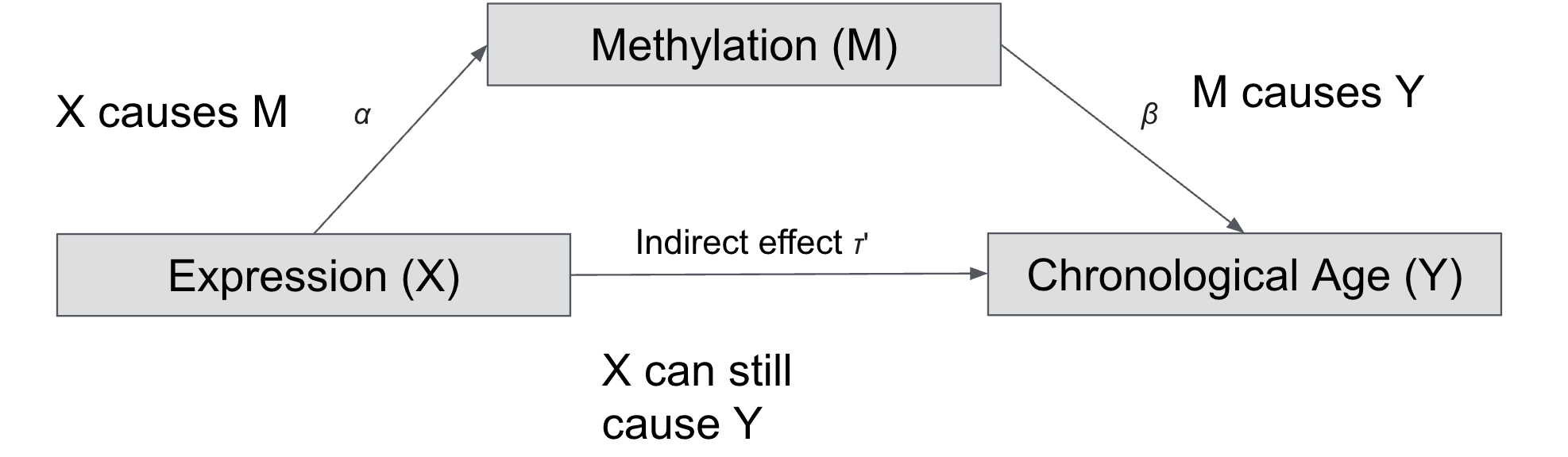
In other words, the change in expression drive changes in methylation level which further drive the chronological age. This is a typical case of “mediation” analysis where methylation is a mediator that explains the chronological age.
We will do a toy example trying to understand how to test if a variable has a “mediating” effect.
The goal of mediation analysis is not to draw causality but to show that possibly the independent variable influences the mediator variable that influences the final variable.
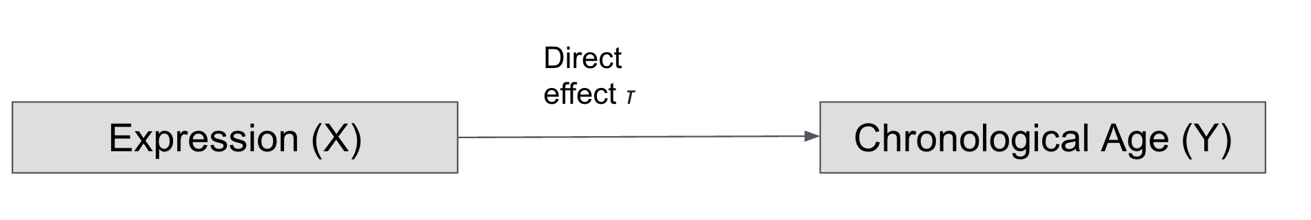
There are multiple steps involved in doing a mediation analysis. here are three steps of regression involved: \(X \longrightarrow Y\) , \(X \longrightarrow M\) and \(X+M \longrightarrow Y\).
We try to estimate the total effect \(Y = \gamma_1 + \tau X + \epsilon_1\)
We will read the data first:
data <- read.csv("mediation_data.csv")
head(data) X M Y
1 6 5 6
2 7 5 5
3 7 7 4
4 8 4 8
5 4 3 5
6 4 4 7library(ggplot2)
library(patchwork)
p1 <- ggplot(data, aes(x = X, y = Y)) +
geom_point() +
theme_minimal()
p1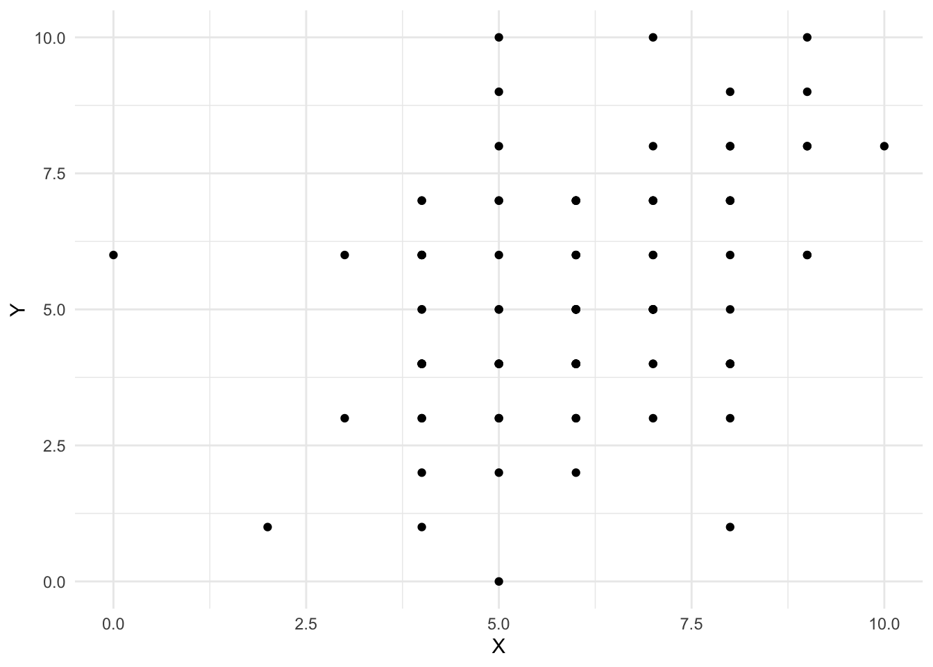
p2 <- ggplot(data, aes(x = X, y = M)) +
  geom_point() +
  theme_minimal()
p2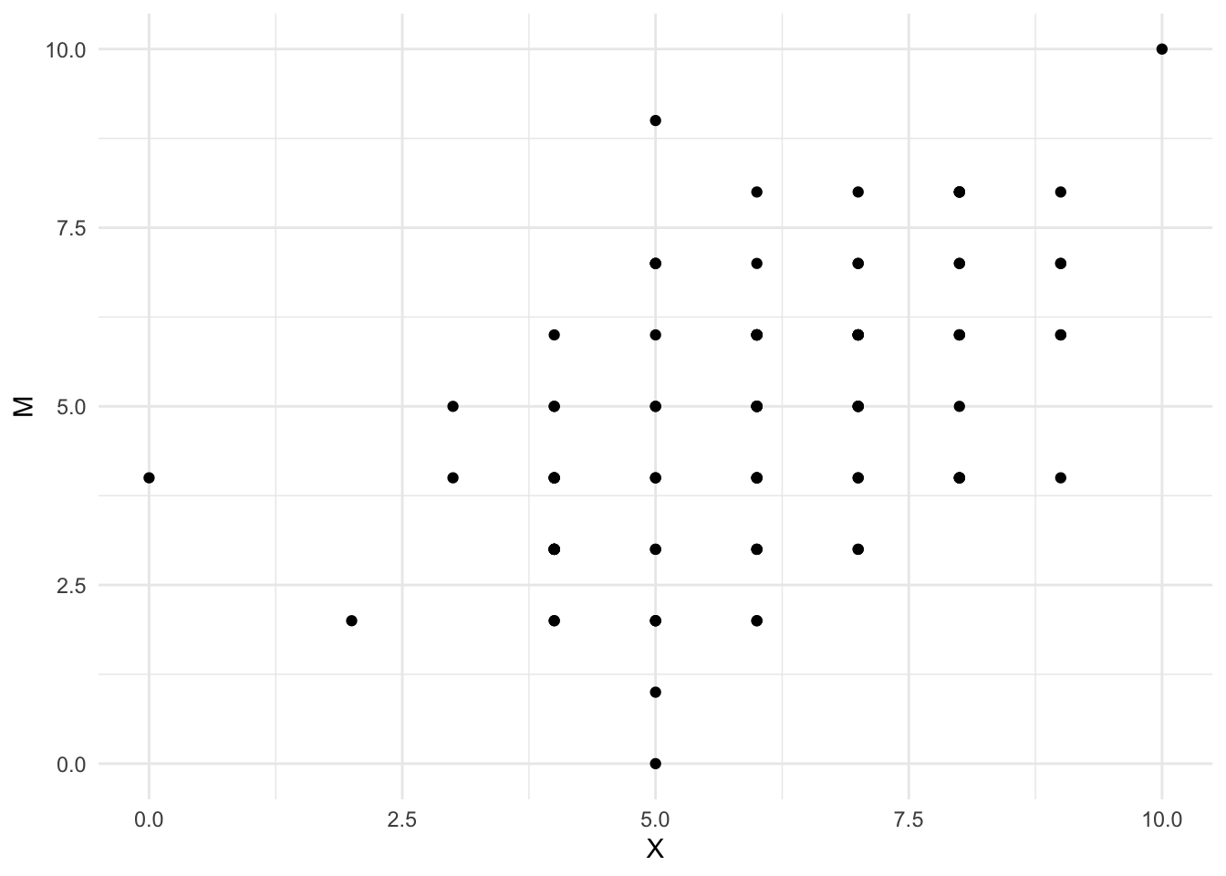
p3 <- ggplot(data, aes(x = M, y = Y)) +
  geom_point() +
  theme_minimal()
p3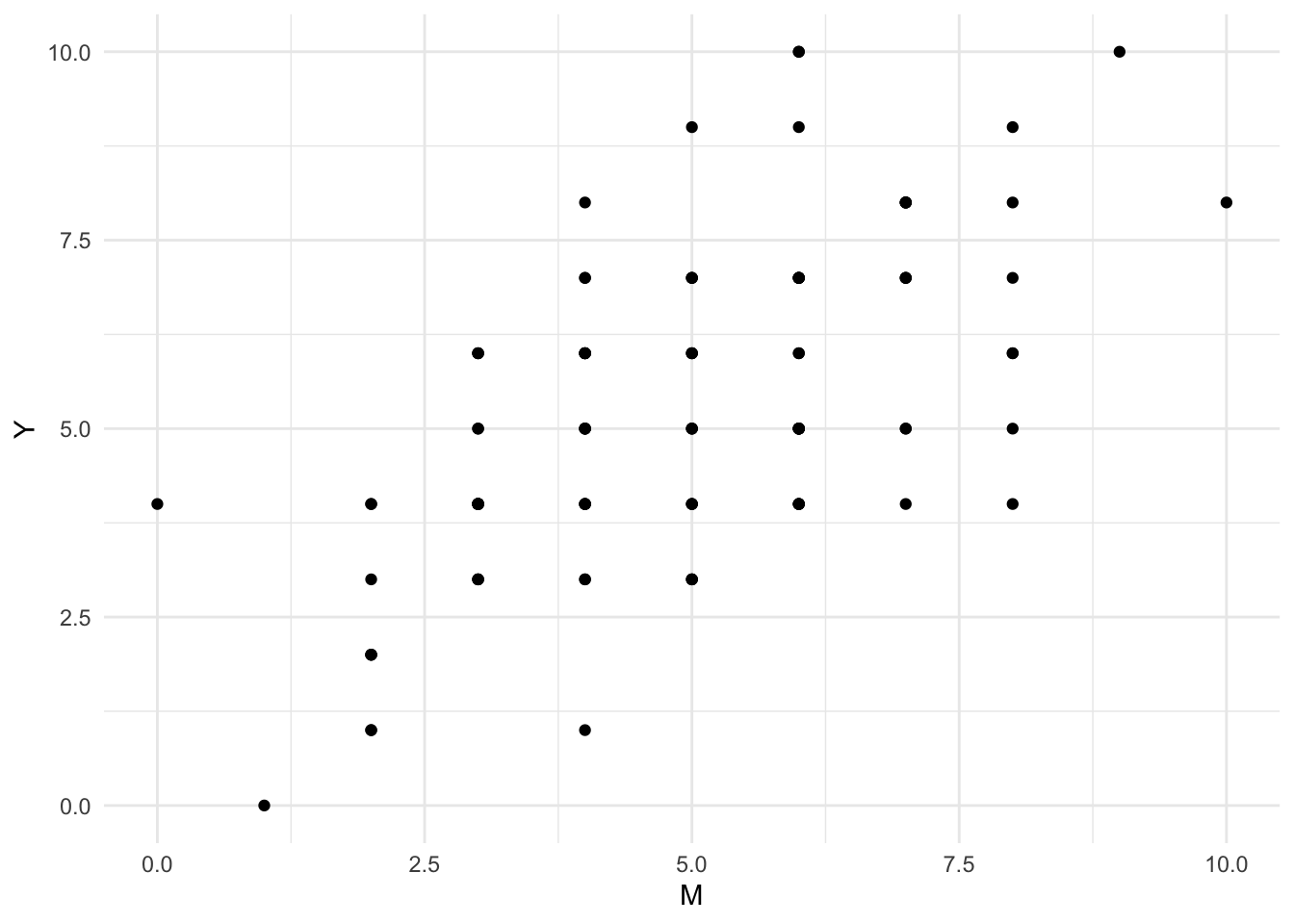
We can visualize them side by side
p1 + p2 + p3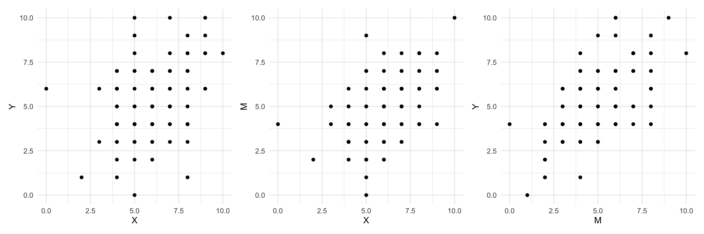
model.1 <- lm(Y ~ X, data)
summary(model.1)
Call:
lm(formula = Y ~ X, data = data)

Residuals:
    Min      1Q  Median      3Q     Max
-5.0262 -1.2340 -0.3282  1.5583  5.1622

Coefficients:
            Estimate Std. Error t value Pr(>|t|)
(Intercept)   2.8572     0.6932   4.122 7.88e-05 ***
X             0.3961     0.1112   3.564 0.000567 ***
---
Signif. codes:  0 '***' 0.001 '**' 0.01 '*' 0.05 '.' 0.1 ' ' 1

Residual standard error: 1.929 on 98 degrees of freedom
Multiple R-squared:  0.1147,    Adjusted R-squared:  0.1057
F-statistic: 12.7 on 1 and 98 DF, p-value: 0.0005671cor(data$X, data$Y)^2[1] 0.114717In step 2, we estimate the following relationship: \(M = \gamma_2 + \alpha X + \epsilon_2\)
model.M <- lm(M ~ X, data)
summary(model.M)
Call:
lm(formula = M ~ X, data = data)

Residuals:
    Min      1Q  Median      3Q     Max
-4.3046 -0.8656  0.1344  1.1344  4.6954

Coefficients:
            Estimate Std. Error t value Pr(>|t|)
(Intercept)  1.49952    0.58920   2.545   0.0125 *
X            0.56102    0.09448   5.938 4.39e-08 ***
---
Signif. codes:  0 '***' 0.001 '**' 0.01 '*' 0.05 '.' 0.1 ' ' 1

Residual standard error: 1.639 on 98 degrees of freedom
Multiple R-squared:  0.2646,    Adjusted R-squared:  0.2571
F-statistic: 35.26 on 1 and 98 DF, p-value: 4.391e-08In step 3, we estimate, if the mediator \(M\) has an effect on \(Y\) after controlling for \(X\): \(Y=\gamma_3 + \tau' X + \beta M + \epsilon_3\)
model.Y <- lm(Y ~ X + M, data)
summary(model.Y)
Call:
lm(formula = Y ~ X + M, data = data)

Residuals:
    Min      1Q  Median      3Q     Max
-3.7631 -1.2393  0.0308  1.0832  4.0055

Coefficients:
            Estimate Std. Error t value Pr(>|t|)
(Intercept)   1.9043     0.6055   3.145   0.0022 **
X             0.0396     0.1096   0.361   0.7187
M             0.6355     0.1005   6.321 7.92e-09 ***
---
Signif. codes:  0 '***' 0.001 '**' 0.01 '*' 0.05 '.' 0.1 ' ' 1

Residual standard error: 1.631 on 97 degrees of freedom
Multiple R-squared:  0.373, Adjusted R-squared:  0.3601
F-statistic: 28.85 on 2 and 97 DF,  p-value: 1.471e-10
After the three steps, if the effect of \(X\) on \(Y\) is reduced after including \(M\) in the model, then we can say that \(M\) is a mediator. We can infer this by comparing the coefficients of \(X\) in model 1 and model 3. To test the significance of the mediation effect, we can use the Sobel test or preferably the bootstrapping method.
We will use the mediate() method to do the bootstrapping method (over the Sobel method which is more conservative). mediate() takes two arguments, the two models \(X \longrightarrow M\) and \(X +M \longrightarrow Y\) along with the treatment variable and mediator variable.
library(mediation)Loading required package: MASS
Attaching package: 'MASS'The following object is masked from 'package:patchwork':
areaLoading required package: MatrixLoading required package: mvtnormLoading required package: sandwichmediation: Causal Mediation Analysis
Version: 4.5.0results <- mediate(
model.m = model.M,
model.y = model.Y,
treat = "X", mediator = "M",
boot = TRUE, sims = 500
)Running nonparametric bootstrapsummary(results)
Causal Mediation Analysis

Nonparametric Bootstrap Confidence Intervals with the Percentile Method

               Estimate 95% CI Lower 95% CI Upper p-value
ACME             0.3565       0.2215         0.52  <2e-16 ***
ADE              0.0396      -0.1985         0.30    0.77
Total Effect     0.3961       0.1698         0.64  <2e-16 ***
Prop. Mediated   0.9000       0.4856         1.92  <2e-16 ***
---
Signif. codes:  0 '***' 0.001 '**' 0.01 '*' 0.05 '.' 0.1 ' ' 1

Sample Size Used: 100


Simulations: 500
Total effect of X on Y is 0.3961 (ACME)
Direct effect of X on Y after taking account into M is 0.0396 (ADE), this is the coefficient \(\tau'\) in the Step 3 model.
The mediation effect (ACME) is the total effect minus the direct effect (0.3961 - 0.0396 = 0.3565), which is also equals to the product of coeffiecient \(\alpha\) of \(X\) in the second step and coefficient of \(\beta\) of \(M\) in the step or 0.56102 * 0.6355 = 0.3565.
We can also run Sobel’s test using the multilevel package:
library(multilevel)Loading required package: nlmefit <- sobel(pred = data$X, med = data$M, out = data$Y)
fit$`Mod1: Y~X`
Estimate Std. Error t value Pr(>|t|)
(Intercept) 2.8572046 0.6932130 4.121684 7.875771e-05
pred 0.3961261 0.1111598 3.563574 5.671128e-04
$`Mod2: Y~X+M`
Estimate Std. Error t value Pr(>|t|)
(Intercept) 1.90426882 0.6054585 3.145168 2.203831e-03
pred 0.03960392 0.1096484 0.361190 7.187429e-01
med 0.63549459 0.1005339 6.321194 7.922642e-09
$`Mod3: M~X`
Estimate Std. Error t value Pr(>|t|)
(Intercept) 1.4995183 0.58919773 2.545017 1.248749e-02
pred 0.5610153 0.09448048 5.937897 4.391362e-08
$Indirect.Effect
[1] 0.3565222
$SE
[1] 0.08237781
$z.value
[1] 4.327891
$N
[1] 100or the bda package:
library(bda)Loading required package: bootbda - 18.3.2fit <- mediation.test(mv = data$M, iv = data$Y, dv = data$X)
fit Sobel Aroian Goodman
z.value 3.8517605206 3.8273091741 3.8766865692
p.value 0.0001172717 0.0001295517 0.0001058886