Linear Models

Saket Choudhary

DH801 Biostatistics in Healthcare · IIT Bombay

Monday, 5th October 2026

Is this baby growing well?

Late in pregnancy, an obstetrician wants to know whether the fetus is too small. A growth-restricted baby may need closer monitoring or an early delivery
You can’t put a fetus on a scale –> You need something you can measure, from the mother, that tracks the fetus
1960s answer: measure a hormone in the mother’s urine that the fetus itself helps to make

Question: Can a urine test taken before delivery tell us how big the baby will be?

Estriol: a hormone the fetus helps make

Estriol (E3) is one of the three main oestrogens (with estrone E1 and estradiol E2). It is usually not found outside pregnancy. In pregnancy its synthesis takes three organs, two of them fetal:

fetal adrenal → fetal liver → placenta → maternal blood → urine

Most pregnancy estriol is built from fetal precursors, so it depends on a working fetus and a working placenta
A bigger, healthier feto-placental unit should make more of it. Hence, Low maternal estriol = warning sign

The data

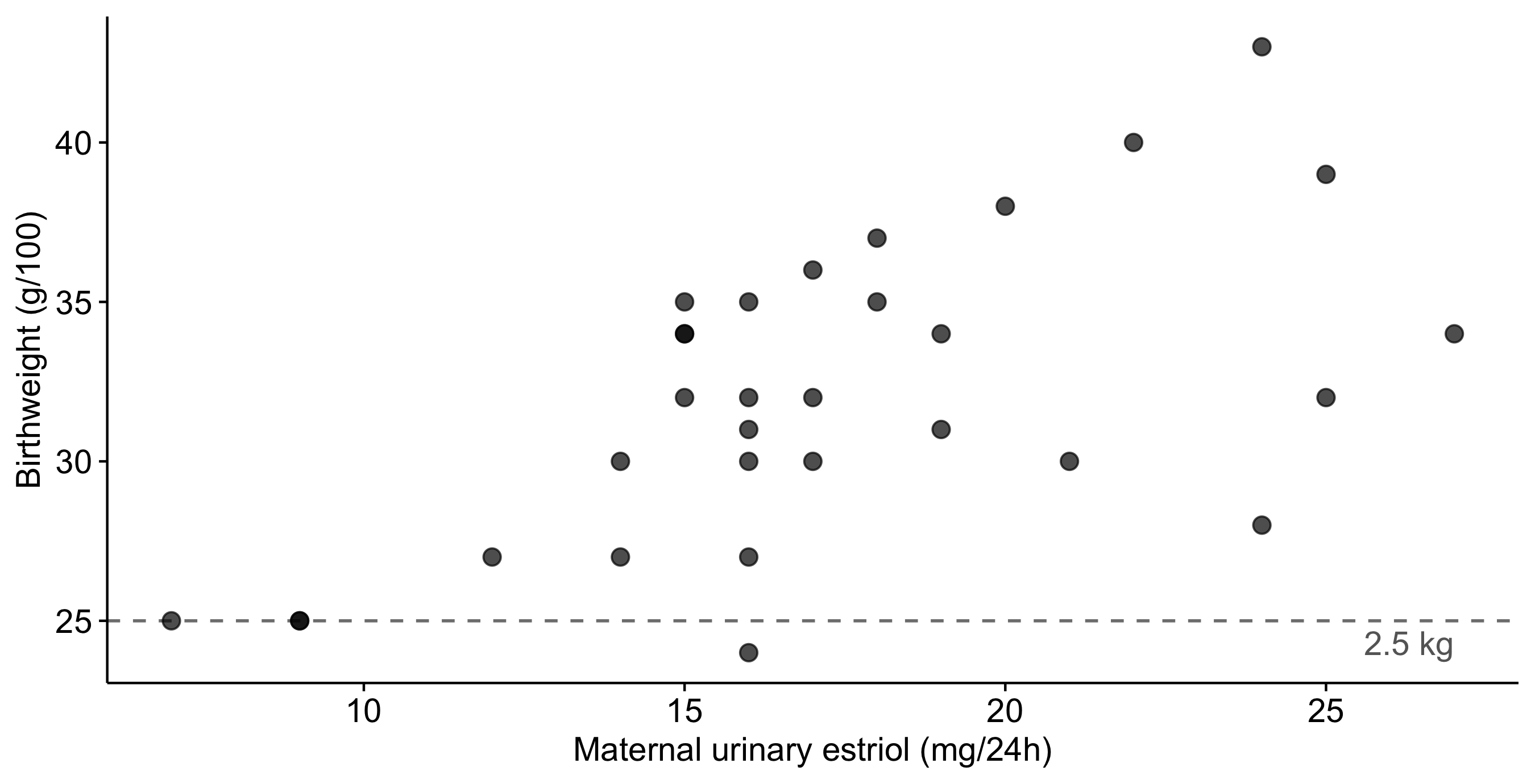
31 pregnancies. Birthweight is in units of 100 g, so 25 = 2.5 kg, the usual low-birthweight cut-off
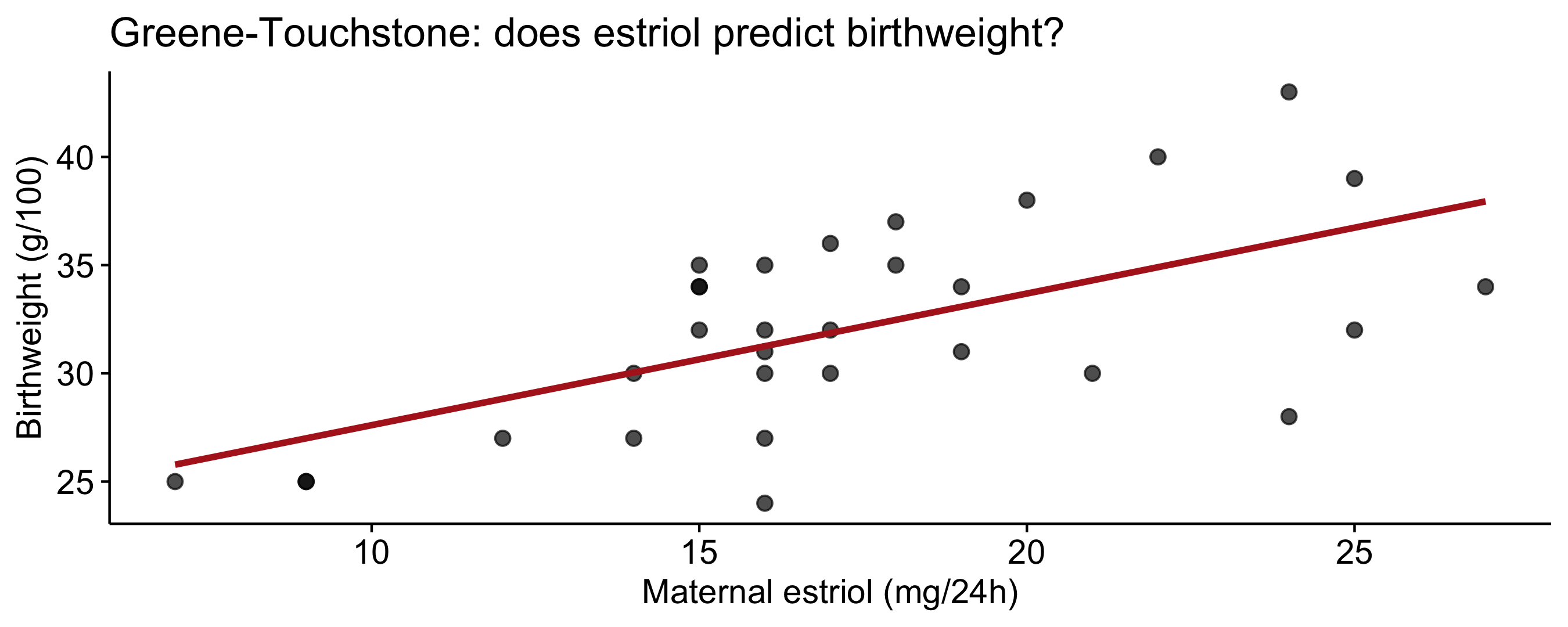
Higher estriol tends to go with heavier babies, but the cloud is wide

How should we model it?

The obstetrician’s questions:

Is there a real relationship, or could this pattern be noise?
How many grams of birthweight go with each extra mg/24h of estriol?
A mother’s estriol is 10 mg/24h. What birthweight should we expect, and how sure are we about this baby?
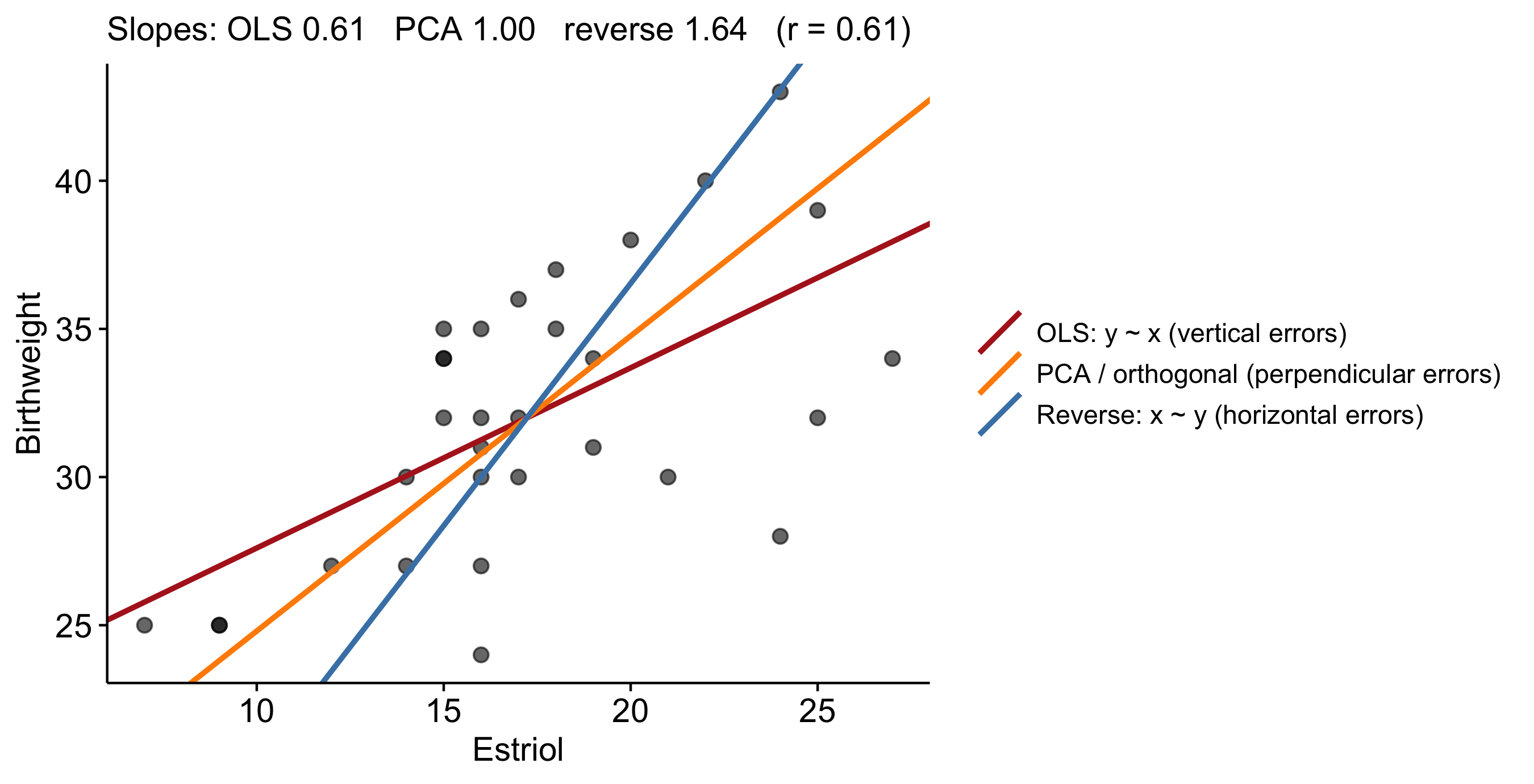
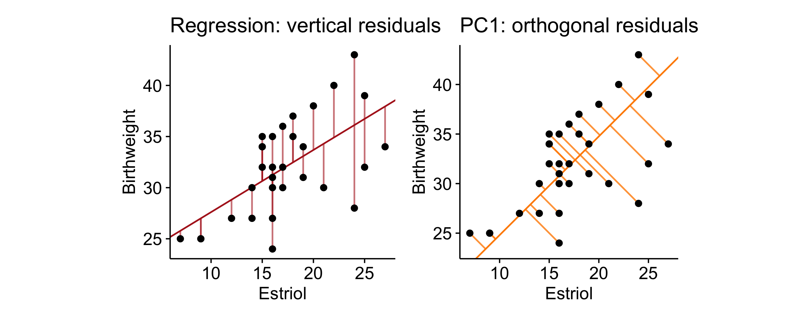
There are many lines through a cloud. Which one, and why?
Does it still hold once we account for other things (gestational age, maternal smoking)?

How should we model it?

Tools you already:

The correlation \(r\) answers 1, but not 2 or 3
Splitting estriol into “low” and “high” and running a two-sample \(t\)-test answers a cruder version of 1 and throws information away
Drawing a line by eye answers 2 and 3, but everyone can draw a different line

Today: one model, \(\;\text{birthweight} = \beta_0 + \beta_1\,\text{estriol} + \varepsilon\), answers 1-4. Adding predictors to it answers 5, and the \(t\)-test turns out to be a special case of it.

Regression models a conditional distribution

Data: pairs \((x_i, y_i)\), \(i = 1,\dots,n\). Goal: describe how the distribution of \(Y\) changes with \(x\), most often its mean \[\mu(x) = \mathbb{E}[Y \mid X = x]\]
“Regression” comes from Galton (1886): tall parents have children who are, on average, tall but less extreme, a “regression towards mediocrity” (more on this soon)
The asymmetry matters: we model \(Y \mid X\), not the joint distribution of \((X, Y)\). \(X\) is treated as known/fixed

The linear model in matrix form

\[ \underbrace{\begin{pmatrix} y_1\\ \vdots\\ y_n\end{pmatrix}}_{\mathbf y} = \underbrace{\begin{pmatrix} 1 & x_{11} & \cdots & x_{1,p-1}\\ \vdots & & & \vdots\\ 1 & x_{n1} & \cdots & x_{n,p-1}\end{pmatrix}}_{\mathbf X\ (n\times p)} \underbrace{\begin{pmatrix} \beta_0\\ \vdots\\ \beta_{p-1}\end{pmatrix}}_{\boldsymbol\beta} + \underbrace{\begin{pmatrix} \varepsilon_1\\ \vdots\\ \varepsilon_n\end{pmatrix}}_{\boldsymbol\varepsilon} \]

Linear means linear in \(\boldsymbol\beta\), not in \(x\). All of these are linear models:
- \(y = \beta_0 + \beta_1 x + \beta_2 x^2 + \varepsilon\) (polynomial)
- \(y = \beta_0 + \beta_1 \log x + \varepsilon\)
- \(y = \beta_0 + \sum_k \beta_k B_k(x) + \varepsilon\) (splines)
- \(y = \beta_0 + \beta_1 \mathbb{1}[\text{treated}] + \varepsilon\) (a two-group comparison!)
Not linear: \(y = \beta_0 e^{\beta_1 x} + \varepsilon\) (but see GLMs)
\(p\) = number of columns of \(\mathbf X\) including the intercept

Assumptions of a linear model

	Assumption	Outcome
A1	\(\mathbb{E}[\boldsymbol\varepsilon \mid \mathbf X] = \mathbf 0\) (mean model is correct)	\(\hat{\boldsymbol\beta}\) is unbiased
A2	\(\mathbf X\) has full column rank \(p\)	\(\hat{\boldsymbol\beta}\) is unique
A3	\(\operatorname{Var}(\boldsymbol\varepsilon \mid \mathbf X) = \sigma^2 \mathbf I\) (equal variance, uncorrelated)	Usual SE formula is right
A4	\(\boldsymbol\varepsilon \mid \mathbf X \sim N(\mathbf 0, \sigma^2\mathbf I)\)	Exact \(t\) and \(F\) tests at any \(n\); OLS = MLE

LINE: L = Linear (A1), I = Independent and E = Equal variance (A3), N = Normality (A4) (strictly, A3 only needs uncorrelated errors; “independent” is stronger, and the two coincide under A4)
Not assumed: \(Y\) marginally normal; \(X\) normal; \(X\) random at all
Large \(n\): by the CLT, \(\hat{\boldsymbol\beta}\) is approximately normal without A4. Normality matters most for small samples and for prediction intervals
Violating A3 leaves \(\hat{\boldsymbol\beta}\) unbiased but makes the standard errors wrong (fix: GLM)

Least squares

Choose \(\boldsymbol\beta\) to minimise the residual sum of squares \[\text{RSS}(\boldsymbol\beta) = \sum_{i=1}^n (y_i - \mathbf x_i^\top\boldsymbol\beta)^2 = \lVert \mathbf y - \mathbf X\boldsymbol\beta\rVert^2\]

Set the gradient to zero: \[\nabla_{\boldsymbol\beta}\,\text{RSS} = -2\mathbf X^\top(\mathbf y - \mathbf X\boldsymbol\beta) = \mathbf 0 \quad\Longrightarrow\quad \underbrace{\mathbf X^\top\mathbf X\,\hat{\boldsymbol\beta} = \mathbf X^\top\mathbf y}_{\text{normal equations}}\] \[\hat{\boldsymbol\beta} = (\mathbf X^\top\mathbf X)^{-1}\mathbf X^\top\mathbf y\]

Simple regression (\(p = 2\)): \[\hat\beta_1 = \frac{S_{xy}}{S_{xx}} = \frac{\sum(x_i-\bar x)(y_i-\bar y)}{\sum (x_i-\bar x)^2} = r\,\frac{s_y}{s_x}, \qquad \hat\beta_0 = \bar y - \hat\beta_1\bar x\]

The fitted line always passes through \((\bar x, \bar y)\)
The slope is the correlation, rescaled into the units of \(y\) per unit of \(x\)

X <- cbind(1, estriol_df$estriol); y <- estriol_df$birthweight
solve(t(X) %*% X, t(X) %*% y) |> t()          # normal equations by hand

         [,1]      [,2]
[1,] 21.52343 0.6081905

coef(lm(birthweight ~ estriol, data = estriol_df))

(Intercept)     estriol 
 21.5234286   0.6081905

Least squares is a projection

\[\hat{\mathbf y} = \mathbf X\hat{\boldsymbol\beta} = \underbrace{\mathbf X(\mathbf X^\top\mathbf X)^{-1}\mathbf X^\top}_{\mathbf H\ \text{(hat matrix)}}\mathbf y, \qquad \mathbf e = \mathbf y - \hat{\mathbf y} = (\mathbf I - \mathbf H)\mathbf y\]

\(\mathbf H\) is symmetric and idempotent (\(\mathbf H^2 = \mathbf H\)): the orthogonal projection of \(\mathbf y \in \mathbb R^n\) onto the column space of \(\mathbf X\)
The normal equations say \(\mathbf X^\top\mathbf e = \mathbf 0\): residuals are orthogonal to every predictor. With an intercept this gives \(\sum e_i = 0\), \(\sum x_{ij} e_i = 0\), \(\sum \hat y_i e_i = 0\)
Pythagoras in \(\mathbb R^n\) (for a model with an intercept, so \(\mathbf 1\) is in the column space of \(\mathbf X\)): \[\underbrace{\lVert\mathbf y - \bar y\mathbf 1\rVert^2}_{\text{TSS}} = \underbrace{\lVert\hat{\mathbf y} - \bar y\mathbf 1\rVert^2}_{\text{SS}_{\text{reg}}} + \underbrace{\lVert\mathbf e\rVert^2}_{\text{RSS}}\]
\(\operatorname{tr}(\mathbf H) = p\), \(\operatorname{tr}(\mathbf I - \mathbf H) = n - p\)
These above traces are the degrees of freedom: \(\mathbf y\) is in \(n\) dimensions, the fit uses \(p\), and the residuals live in the remaining \(n-p\)

Why squares? Least squares = maximum likelihood

If \(y_i \mid \mathbf x_i \sim N(\mathbf x_i^\top\boldsymbol\beta, \sigma^2)\) independently: \[\ell(\boldsymbol\beta, \sigma^2) = -\frac n2\log(2\pi\sigma^2) - \frac{1}{2\sigma^2}\underbrace{\sum_i (y_i - \mathbf x_i^\top\boldsymbol\beta)^2}_{\text{RSS}(\boldsymbol\beta)}\]

For any \(\sigma^2\), maximising \(\ell\) over \(\boldsymbol\beta\) is minimising RSS, so OLS = MLE under Gaussian errors
MLE of variance: \(\hat\sigma^2_{\text{ML}} = \text{RSS}/n\), which is biased: \(\mathbb E[\text{RSS}] = \sigma^2\operatorname{tr}(\mathbf I - \mathbf H) = \sigma^2(n-p)\). So we use \(s^2 = \text{RSS}/(n-p)\) (R’s “residual standard error” is \(s\))

Why least squares?

Changing the noise model changes the loss:

Error distribution	Loss minimised	Targets
Gaussian	\(\sum (y_i - \mathbf x_i^\top\boldsymbol\beta)^2\)	conditional mean
Laplace	\(\sum \lvert y_i - \mathbf x_i^\top\boldsymbol\beta\rvert\)	conditional median (quantile regression)
Bernoulli / Poisson	\(-\sum \log f(y_i;\mu_i)\)	mean on a link scale (GLMs)

Different ways of doing a linear fit

All three pass through \((\bar x, \bar y)\). They differ only in which distance they make small
Note \(\hat\beta_{y\sim x} \times \hat\beta_{x\sim y} = r^2\): the two regression lines coincide only if \(|r| = 1\)

Objective functions

Method	Minimises	Slope (in \(y\)-vs-\(x\) plane)
OLS \(y \sim x\)	\(\sum_i (y_i - \beta_0 - \beta_1 x_i)^2\) (vertical)	\(s_{xy}/s_{xx}\)
OLS \(x \sim y\)	\(\sum_i (x_i - \gamma_0 - \gamma_1 y_i)^2\) (horizontal)	\(s_{yy}/s_{xy}\)
PCA / total least squares	\(\sum_i \dfrac{(y_i - \beta_0 - \beta_1 x_i)^2}{1+\beta_1^2}\) (perpendicular)	\(\dfrac{s_{yy}-s_{xx}+\sqrt{(s_{yy}-s_{xx})^2+4s_{xy}^2}}{2s_{xy}}\)

PC1 is the leading eigenvector of the sample covariance matrix \(\mathbf S\); the formula above is that eigenvector’s slope in 2D

Different error models answer different questions

Linear regression

\[y_i = \mathbf x_i^\top\boldsymbol\beta + \varepsilon_i\]

One variable is the response; predictors are observed without error
All noise is in \(y\), so the residual is measured vertically
Asymmetric: \(y\sim x\) and \(x\sim y\) answer different questions
Target: \(\mathbb E[Y\mid X]\), i.e. prediction / adjusted association
Equivariant to units: rescale \(x\) and the slope rescales accordingly

PCA

\[\mathbf x_i = \boldsymbol\mu + \mathbf W\mathbf z_i + \boldsymbol\varepsilon_i,\quad \boldsymbol\varepsilon_i\sim N(\mathbf 0,\sigma^2\mathbf I)\]

No response: all coordinates are treated alike
The “predictors” \(\mathbf z_i\) (scores) are latent, estimated jointly with \(\mathbf W\)
Noise is isotropic in every coordinate, so error is measured perpendicular to the subspace
Target: best rank-\(k\) reconstruction, \(\min_{\operatorname{rank}(\mathbf L)\le k}\lVert \mathbf X_c - \mathbf L\rVert_F^2\)
Not scale invariant: change g to kg and PC1 changes direction. Hence scale = TRUE

Regression is a supervised linear model (observed inputs, one noisy output)
PCA is an unsupervised linear model (latent inputs, all outputs noisy). :::

Sampling distribution of \(\hat{\boldsymbol\beta}\)

Substitute \(\mathbf y = \mathbf X\boldsymbol\beta + \boldsymbol\varepsilon\): \[\hat{\boldsymbol\beta} = (\mathbf X^\top\mathbf X)^{-1}\mathbf X^\top\mathbf y = \boldsymbol\beta + (\mathbf X^\top\mathbf X)^{-1}\mathbf X^\top\boldsymbol\varepsilon\]

A1 gives \(\mathbb E[\hat{\boldsymbol\beta}] = \boldsymbol\beta\)
A3 gives \(\operatorname{Var}(\hat{\boldsymbol\beta}) = (\mathbf X^\top\mathbf X)^{-1}\mathbf X^\top(\sigma^2\mathbf I)\mathbf X(\mathbf X^\top\mathbf X)^{-1} = \sigma^2(\mathbf X^\top\mathbf X)^{-1}\)
A4 gives \(\hat{\boldsymbol\beta}\sim N\big(\boldsymbol\beta,\ \sigma^2(\mathbf X^\top\mathbf X)^{-1}\big)\) exactly

Simple regression: \[\operatorname{Var}(\hat\beta_1) = \frac{\sigma^2}{\sum_i (x_i-\bar x)^2},\qquad \operatorname{Var}(\hat\beta_0) = \sigma^2\left(\frac1n + \frac{\bar x^2}{\sum_i(x_i-\bar x)^2}\right)\]

Why a \(t\) distribution?

\(\sigma^2\) is unknown; estimate it by \(s^2 = \text{RSS}/(n-p)\)
Under A4: \(\hat{\boldsymbol\beta}\) depends on \(\mathbf H\mathbf y\), RSS on \((\mathbf I-\mathbf H)\mathbf y\). These are orthogonal projections of a Gaussian vector, so they are independent, and \[\frac{(n-p)s^2}{\sigma^2}\sim\chi^2_{n-p}\]
Therefore \[T_j = \frac{\hat\beta_j - \beta_j}{\widehat{\text{SE}}(\hat\beta_j)} \sim t_{n-p},\qquad \widehat{\text{SE}}(\hat\beta_j) = s\sqrt{[(\mathbf X^\top\mathbf X)^{-1}]_{jj}}\] (\(N(0,1)\) divided by \(\sqrt{\chi^2_{n-p}/(n-p)}\), independent: that is the definition of \(t_{n-p}\))
If \(\sigma\) were known, \(T_j\) would be exactly \(N(0,1)\): the \(z\)-test. As \(n\to\infty\), \(t_{n-p}\to N(0,1)\) anyway

fit <- lm(birthweight ~ estriol, data = estriol_df)
summary(fit)$coefficients

              Estimate Std. Error  t value     Pr(>|t|)
(Intercept) 21.5234286  2.6204170 8.213742 4.679259e-09
estriol      0.6081905  0.1468117 4.142656 2.712299e-04

confint(fit)   # beta_hat +/- qt(0.975, n - 2) * SE

                 2.5 %     97.5 %
(Intercept) 16.1640740 26.8827831
estriol      0.3079268  0.9084542