Chapter 3 - Linear regression: the basics
import warnings

import pandas as pd
import proplot as plot
import seaborn as sns
import statsmodels.api as sm
import statsmodels.formula.api as smf
from scipy import stats

warnings.filterwarnings("ignore")

%pylab inline


plt.rcParams["axes.labelweight"] = "bold"
plt.rcParams["font.weight"] = "bold"
Populating the interactive namespace from numpy and matplotlib
kidiq_df = pd.read_csv("../data/kidiq.tsv.gz", sep="\t")
kidiq_df.head()
| kid_score | mom_hs | mom_iq | mom_work | mom_age | |
|---|---|---|---|---|---|
| 0 | 65 | 1.0 | 121.117529 | 4 | 27 |
| 1 | 98 | 1.0 | 89.361882 | 4 | 25 |
| 2 | 85 | 1.0 | 115.443165 | 4 | 27 |
| 3 | 83 | 1.0 | 99.449639 | 3 | 25 |
| 4 | 115 | 1.0 | 92.745710 | 4 | 27 |
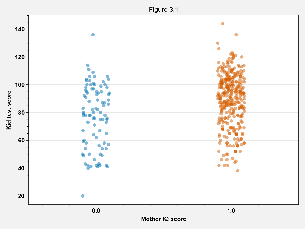
The data represents cognitive test-scores of three- and four-year-old children given characteristics of their mothers, using data from a survey of adult American women and their children.
Figure 3.1
fig, ax = plt.subplots()
sns.stripplot(x="mom_hs", y="kid_score", data=kidiq_df, ax=ax, alpha=0.5)
ax.set_xlabel("Mother IQ score")
ax.set_ylabel("Kid test score")
ax.set_title("Figure 3.1")
fig.tight_layout()
One predictor
Binary predictor
model = sm.OLS(kidiq_df["kid_score"], sm.add_constant(kidiq_df[["mom_hs"]]))
model = smf.ols(formula="""kid_score ~ mom_hs""", data=kidiq_df)
results_hs = model.fit()
print(results_hs.summary())
                            OLS Regression Results
==============================================================================
Dep. Variable:              kid_score   R-squared:                       0.056
Model:                            OLS   Adj. R-squared:                  0.054
Method:                 Least Squares   F-statistic:                     25.69
Date:                Sat, 20 Jun 2020   Prob (F-statistic):           5.96e-07
Time:                        22:37:21   Log-Likelihood:                -1911.8
No. Observations:                 434   AIC:                             3828.
Df Residuals:                     432   BIC:                             3836.
Df Model:                           1
Covariance Type:            nonrobust
==============================================================================
                 coef    std err          t      P>|t|      [0.025      0.975]
------------------------------------------------------------------------------
Intercept     77.5484      2.059     37.670      0.000      73.502      81.595
mom_hs        11.7713      2.322      5.069      0.000       7.207      16.336
==============================================================================
Omnibus:                       11.077   Durbin-Watson:                   1.464
Prob(Omnibus):                  0.004   Jarque-Bera (JB):               11.316
Skew:                          -0.373   Prob(JB):                      0.00349
Kurtosis:                       2.738   Cond. No.                         4.11
==============================================================================

Warnings:
[1] Standard Errors assume that the covariance matrix of the errors is correctly specified.
Thus,
This model summarized the difference in average test scores between children of mothers who completed high school against those who did not.
Thus, children whose mothers have completed high school score 12 points higher on average than children of methoers who haven’t.
Continuous predictor
model = smf.ols(formula="""kid_score ~ mom_iq + 1""", data=kidiq_df)
results_iq = model.fit()
print(results_iq.summary())
                            OLS Regression Results
==============================================================================
Dep. Variable:              kid_score   R-squared:                       0.201
Model:                            OLS   Adj. R-squared:                  0.199
Method:                 Least Squares   F-statistic:                     108.6
Date:                Sat, 20 Jun 2020   Prob (F-statistic):           7.66e-23
Time:                        22:37:21   Log-Likelihood:                -1875.6
No. Observations:                 434   AIC:                             3755.
Df Residuals:                     432   BIC:                             3763.
Df Model:                           1
Covariance Type:            nonrobust
==============================================================================
                 coef    std err          t      P>|t|      [0.025      0.975]
------------------------------------------------------------------------------
Intercept     25.7998      5.917      4.360      0.000      14.169      37.430
mom_iq         0.6100      0.059     10.423      0.000       0.495       0.725
==============================================================================
Omnibus:                        7.545   Durbin-Watson:                   1.645
Prob(Omnibus):                  0.023   Jarque-Bera (JB):                7.735
Skew:                          -0.324   Prob(JB):                       0.0209
Kurtosis:                       2.919   Cond. No.                         682.
==============================================================================

Warnings:
[1] Standard Errors assume that the covariance matrix of the errors is correctly specified.
results_iq_hs = smf.ols(
    formula="""kid_score ~ mom_iq + mom_hs + 1""", data=kidiq_df
).fit()
print(results_iq_hs.summary())
                            OLS Regression Results
==============================================================================
Dep. Variable:              kid_score   R-squared:                       0.214
Model:                            OLS   Adj. R-squared:                  0.210
Method:                 Least Squares   F-statistic:                     58.72
Date:                Sat, 20 Jun 2020   Prob (F-statistic):           2.79e-23
Time:                        22:37:21   Log-Likelihood:                -1872.0
No. Observations:                 434   AIC:                             3750.
Df Residuals:                     431   BIC:                             3762.
Df Model:                           2
Covariance Type:            nonrobust
==============================================================================
                 coef    std err          t      P>|t|      [0.025      0.975]
------------------------------------------------------------------------------
Intercept     25.7315      5.875      4.380      0.000      14.184      37.279
mom_iq         0.5639      0.061      9.309      0.000       0.445       0.683
mom_hs         5.9501      2.212      2.690      0.007       1.603      10.297
==============================================================================
Omnibus:                        7.327   Durbin-Watson:                   1.625
Prob(Omnibus):                  0.026   Jarque-Bera (JB):                7.530
Skew:                          -0.313   Prob(JB):                       0.0232
Kurtosis:                       2.845   Cond. No.                         683.
==============================================================================

Warnings:
[1] Standard Errors assume that the covariance matrix of the errors is correctly specified.
Interpretation:
Intercept (26): If a child had a mother who did not complete high school and an IQ of 0, then we would predict this child’s test score to be 26.
Coeff of mom_hs (6): If the mothers had same IQ, then a child whose mother went to high school will have 6 additional points as compared to the child whose mother did not go to high school.
Coeff of mom_iq (0.6): Comparing children with same value of mom_hs, if mother IQ differs by 1 then children are expected to have a difference of 0.6 points.
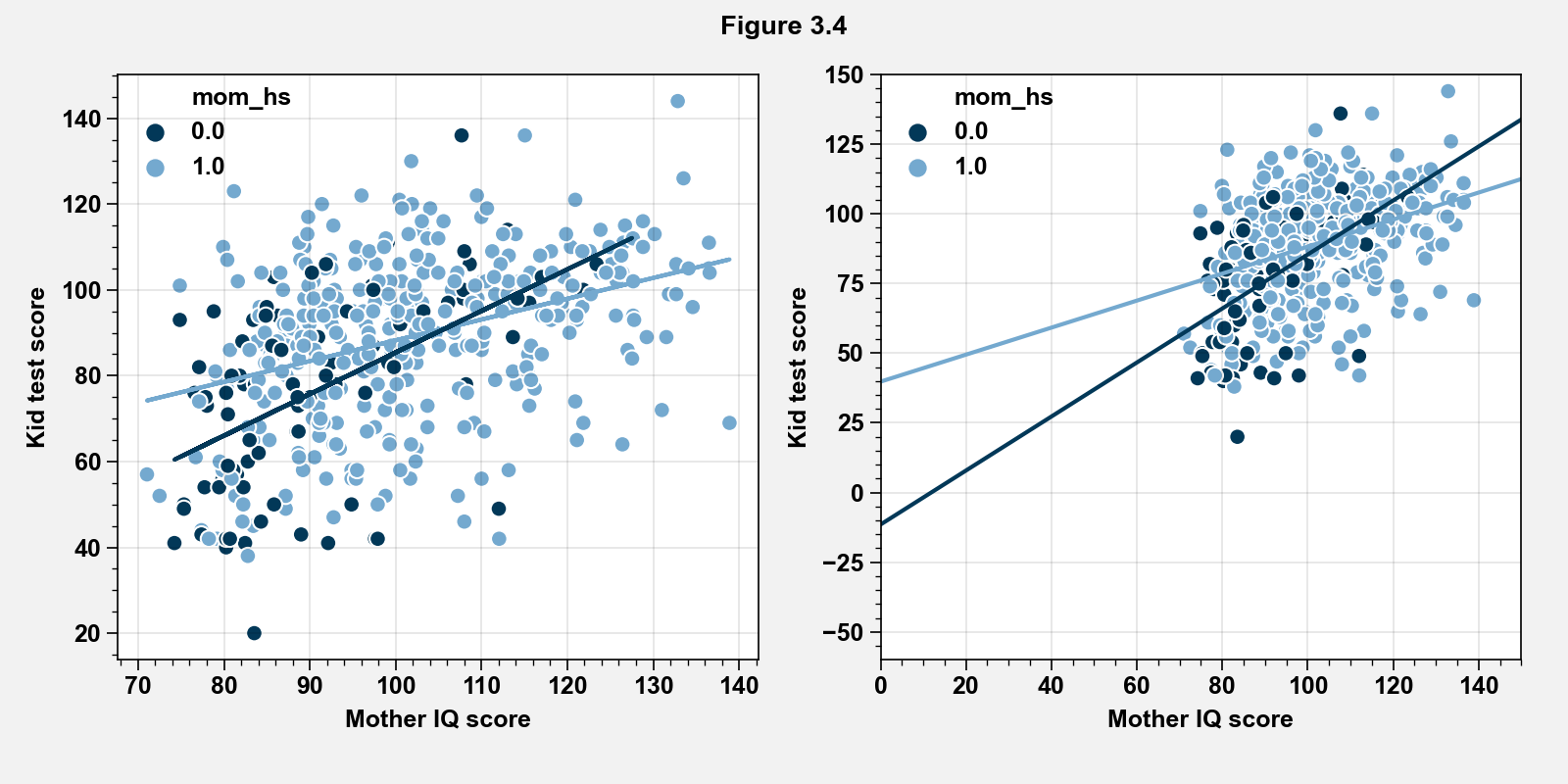
Interaction
results_iq_hs_interaction = smf.ols(
    formula="""kid_score ~ mom_hs + mom_iq + mom_hs:mom_iq""", data=kidiq_df
).fit()
print(results_iq_hs_interaction.summary())
                            OLS Regression Results
==============================================================================
Dep. Variable:              kid_score   R-squared:                       0.230
Model:                            OLS   Adj. R-squared:                  0.225
Method:                 Least Squares   F-statistic:                     42.84
Date:                Sat, 20 Jun 2020   Prob (F-statistic):           3.07e-24
Time:                        22:37:21   Log-Likelihood:                -1867.5
No. Observations:                 434   AIC:                             3743.
Df Residuals:                     430   BIC:                             3759.
Df Model:                           3
Covariance Type:            nonrobust
=================================================================================
                    coef    std err          t      P>|t|      [0.025      0.975]
---------------------------------------------------------------------------------
Intercept       -11.4820     13.758     -0.835      0.404     -38.523      15.559
mom_hs           51.2682     15.338      3.343      0.001      21.122      81.414
mom_iq            0.9689      0.148      6.531      0.000       0.677       1.260
mom_hs:mom_iq    -0.4843      0.162     -2.985      0.003      -0.803      -0.165
==============================================================================
Omnibus:                        8.014   Durbin-Watson:                   1.660
Prob(Omnibus):                  0.018   Jarque-Bera (JB):                8.258
Skew:                          -0.333   Prob(JB):                       0.0161
Kurtosis:                       2.887   Cond. No.                     3.10e+03
==============================================================================

Warnings:
[1] Standard Errors assume that the covariance matrix of the errors is correctly specified.
[2] The condition number is large, 3.1e+03. This might indicate that there are
strong multicollinearity or other numerical problems.
Interpretation
Intercept (-12_: Predicted score for children whose mothers did not finish high school and have an IQ of 0. This is impossible scenario.
Coeff of mom_hs: Difference of predicted kids’s score with mothers whose high school status is the same = mothers did not complete high school and had an IQ of 0 and those whose mothers did complete high school but had an IQ of 0
Coeff of mom_iq: Difference of predicted kids’ score with mothers who did not complete high school but whose mothers had an IQ difference of 1.
Coeff of mom_hs:mom_iq: Difference in slope for mom_iq comparing children with mothers who did and did not complete
It is also possible to see the interpretation of the interaction term by breaking it down into two categories: children with mom_hs = 1 and children with mom_hs = 0:
mom_hs = 0: \begin{align*}\mathrm{kid_score} &= -11 + 51.2(0) + 1.1.\mathrm{mom_iq}\ &= -11 + 1.1.\mathrm{mom_iq} \end{align*}
mom_hs = 1: \begin{align*}\mathrm{kid_score} &= -11 + 51.2(1) + 1.1.\mathrm{mom_iq} - 0.5.1.\mathrm{mom_iq}\ &= 40 + 0.6.\mathrm{mom_iq} \end{align*}
kidiq_hs1 = kidiq_df.loc[kidiq_df.mom_hs == 1]
kidiq_hs0 = kidiq_df.loc[kidiq_df.mom_hs == 0]

results_iq_hs_interaction = smf.ols(
    formula="""kid_score ~ mom_hs + mom_iq + mom_hs:mom_iq""", data=kidiq_df
).fit()


line_hs1 = (
    results_iq_hs_interaction.params[0]
    + results_iq_hs_interaction.params[1] * kidiq_hs1["mom_hs"]
    + results_iq_hs_interaction.params[2] * kidiq_hs1["mom_iq"]
    + results_iq_hs_interaction.params[3] * kidiq_hs1["mom_hs"] * kidiq_hs1["mom_iq"]
)
line_hs0 = (
    results_iq_hs_interaction.params[0]
    + results_iq_hs_interaction.params[1] * kidiq_hs0["mom_hs"]
    + results_iq_hs_interaction.params[2] * kidiq_hs0["mom_iq"]
    + results_iq_hs_interaction.params[3] * kidiq_hs0["mom_hs"] * kidiq_hs0["mom_iq"]
)


fig = plt.figure(figsize=(8, 4))
ax = plt.subplot(121)
palette = {0: "#023858", 1: "#74a9cf"}
sns.scatterplot(x="mom_iq", y="kid_score", hue="mom_hs", data=kidiq_df, palette=palette)
ax.plot(kidiq_hs1["mom_iq"], line_hs1, color=palette[1])
ax.plot(kidiq_hs0["mom_iq"], line_hs0, color=palette[0])

ax.set_xlabel("Mother IQ score")
ax.set_ylabel("Kid test score")
ax.legend(frameon=False)

ax = plt.subplot(122)
palette = {0: "#023858", 1: "#74a9cf"}
sns.scatterplot(x="mom_iq", y="kid_score", hue="mom_hs", data=kidiq_df, palette=palette)

ax.set_xlim(0, 150)
ax.set_ylim(-60, 150)

m, b = np.polyfit(kidiq_hs1["mom_iq"], line_hs1, 1)
xpoints = np.linspace(0, 150, 1000)
ax.plot(xpoints, xpoints * m + b, color=palette[1])

m, b = np.polyfit(kidiq_hs0["mom_iq"], line_hs0, 1)
ax.plot(xpoints, xpoints * m + b, color=palette[0])
ax.set_xlabel("Mother IQ score")
ax.set_ylabel("Kid test score")
ax.legend(frameon=False)


fig.suptitle("Figure 3.4")
fig.tight_layout(rect=[0, 0.03, 1, 0.95])
Fitting and summarizing regressions
results_hs_iq = smf.ols(formula="""kid_score ~ mom_hs + mom_iq""", data=kidiq_df).fit()
print(results_hs_iq.summary())
                            OLS Regression Results
==============================================================================
Dep. Variable:              kid_score   R-squared:                       0.214
Model:                            OLS   Adj. R-squared:                  0.210
Method:                 Least Squares   F-statistic:                     58.72
Date:                Sat, 20 Jun 2020   Prob (F-statistic):           2.79e-23
Time:                        22:37:21   Log-Likelihood:                -1872.0
No. Observations:                 434   AIC:                             3750.
Df Residuals:                     431   BIC:                             3762.
Df Model:                           2
Covariance Type:            nonrobust
==============================================================================
                 coef    std err          t      P>|t|      [0.025      0.975]
------------------------------------------------------------------------------
Intercept     25.7315      5.875      4.380      0.000      14.184      37.279
mom_hs         5.9501      2.212      2.690      0.007       1.603      10.297
mom_iq         0.5639      0.061      9.309      0.000       0.445       0.683
==============================================================================
Omnibus:                        7.327   Durbin-Watson:                   1.625
Prob(Omnibus):                  0.026   Jarque-Bera (JB):                7.530
Skew:                          -0.313   Prob(JB):                       0.0232
Kurtosis:                       2.845   Cond. No.                         683.
==============================================================================

Warnings:
[1] Standard Errors assume that the covariance matrix of the errors is correctly specified.
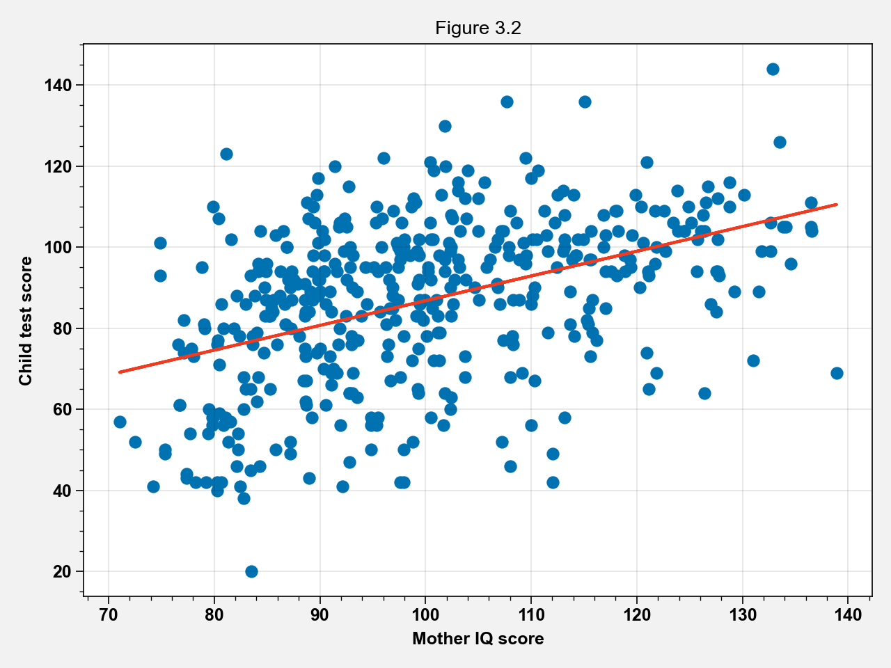
Displaying a regression line as a function of one input variable
results_iq = smf.ols(formula="""kid_score ~ mom_iq""", data=kidiq_df).fit()
print(results_iq.summary())
                            OLS Regression Results
==============================================================================
Dep. Variable:              kid_score   R-squared:                       0.201
Model:                            OLS   Adj. R-squared:                  0.199
Method:                 Least Squares   F-statistic:                     108.6
Date:                Sat, 20 Jun 2020   Prob (F-statistic):           7.66e-23
Time:                        22:37:22   Log-Likelihood:                -1875.6
No. Observations:                 434   AIC:                             3755.
Df Residuals:                     432   BIC:                             3763.
Df Model:                           1
Covariance Type:            nonrobust
==============================================================================
                 coef    std err          t      P>|t|      [0.025      0.975]
------------------------------------------------------------------------------
Intercept     25.7998      5.917      4.360      0.000      14.169      37.430
mom_iq         0.6100      0.059     10.423      0.000       0.495       0.725
==============================================================================
Omnibus:                        7.545   Durbin-Watson:                   1.645
Prob(Omnibus):                  0.023   Jarque-Bera (JB):                7.735
Skew:                          -0.324   Prob(JB):                       0.0209
Kurtosis:                       2.919   Cond. No.                         682.
==============================================================================

Warnings:
[1] Standard Errors assume that the covariance matrix of the errors is correctly specified.
fig, ax = plt.subplots()
ax.scatter(kidiq_df["mom_iq"], kidiq_df["kid_score"])
line = results_iq.params[0] + results_iq.params[1] * kidiq_df["mom_iq"]
ax.plot(kidiq_df["mom_iq"], line, color="#f03b20")
ax.set_title("Figure 3.2")
ax.set_xlabel("Mother IQ score")
ax.set_ylabel("Child test score")
fig.tight_layout()
kidiq_hs1 = kidiq_df.loc[kidiq_df.mom_hs == 1]
kidiq_hs0 = kidiq_df.loc[kidiq_df.mom_hs == 0]
results_iq_hs1 = smf.ols(formula="""kid_score ~ mom_iq + 1""", data=kidiq_hs1).fit()
results_iq_hs0 = smf.ols(formula="""kid_score ~ mom_iq + 1""", data=kidiq_hs0).fit()
results_iq_hs = smf.ols(
formula="""kid_score ~ mom_iq + mom_hs + 1""", data=kidiq_df
).fit()
line_hs1 = results_iq_hs1.params[0] + results_iq_hs1.params[1] * kidiq_hs1["mom_iq"]
line_hs0 = results_iq_hs0.params[0] + results_iq_hs0.params[1] * kidiq_hs0["mom_iq"]
line_hs1 = (
results_iq_hs.params[0]
+ results_iq_hs.params[1] * kidiq_hs1["mom_iq"]
+ results_iq_hs.params[2] * kidiq_hs1["mom_hs"]
)
line_hs0 = (
results_iq_hs.params[0]
+ results_iq_hs.params[1] * kidiq_hs0["mom_iq"]
+ results_iq_hs.params[2] * kidiq_hs0["mom_hs"]
)
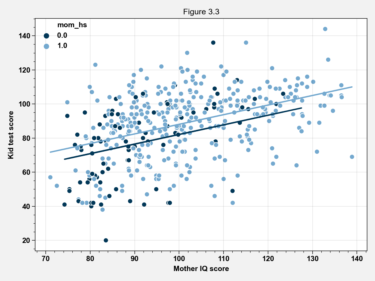
fig, ax = plt.subplots()
palette = {0: "#023858", 1: "#74a9cf"}
sns.scatterplot(x="mom_iq", y="kid_score", hue="mom_hs", data=kidiq_df, palette=palette)
ax.plot(kidiq_hs1["mom_iq"], line_hs1, color=palette[1])
ax.plot(kidiq_hs0["mom_iq"], line_hs0, color=palette[0])
ax.set_xlabel("Mother IQ score")
ax.set_ylabel("Kid test score")
ax.legend(frameon=False)
ax.set_title("Figure 3.3")
fig.tight_layout()
TODO: Displaying uncertainity in the fitted regression
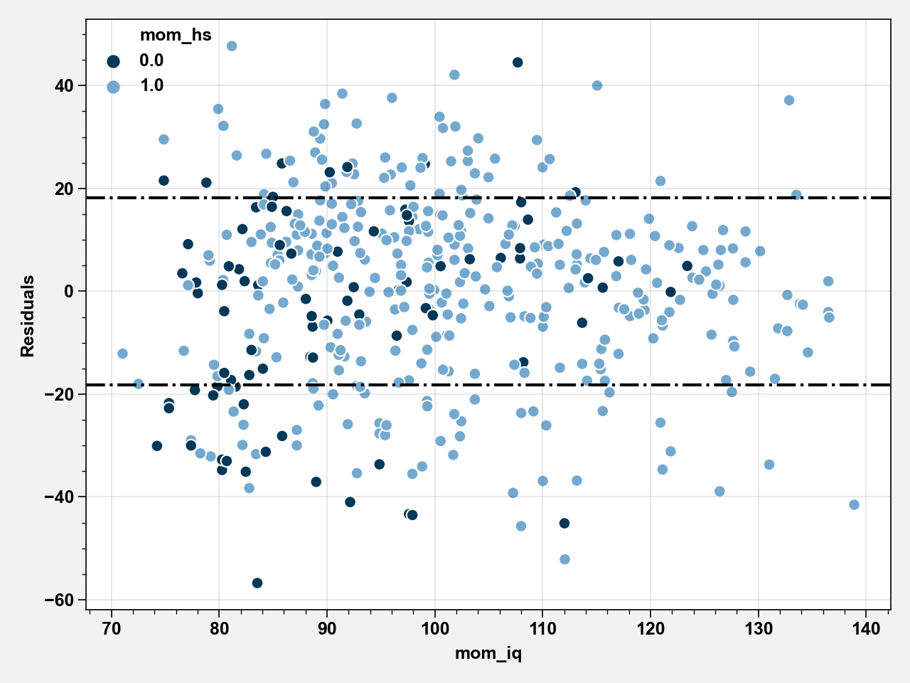
Plotting residuals
results_iq = smf.ols(formula="""kid_score ~ mom_iq""", data=kidiq_df).fit()
kidiq_df["Residuals"] = results_iq.resid
sd = kidiq_df["Residuals"].std()
fig, ax = plt.subplots()
palette = {0: "#023858", 1: "#74a9cf"}
sns.scatterplot(x="mom_iq", y="Residuals", hue="mom_hs", data=kidiq_df, palette=palette)

ax.axhline(y=sd * 1, linestyle="-.", color="black")
ax.axhline(y=sd * -1, linestyle="-.", color="black")
ax.legend(frameon=False)
fig.tight_layout()