set.seed(1000)Lecture 09: Good vs bad model fit
Overview
This notebook demonstrates examples of good and bad linear model fits, including:
- Good fit: Linear relationship with constant variance
- Bad fit examples:
- Non-linear relationship
- Heteroscedasticity (non-constant variance)
- Non-normal residuals
- Influential outliers
Setup
Good fit
A well-fitting linear model with:
- Linear relationship between X and Y
- Constant variance (homoscedasticity)
- Normally distributed residuals
# Good fit
n <- 100
x1 <- rnorm(n, mean = 5, sd = 2)
y1 <- 2 + 3 * x1 + rnorm(n, mean = 0, sd = 2)  # Linear with constant variance
model1 <- lm(y1 ~ x1)

par(mfrow = c(2, 2))
plot(model1, main = "GOOD FIT")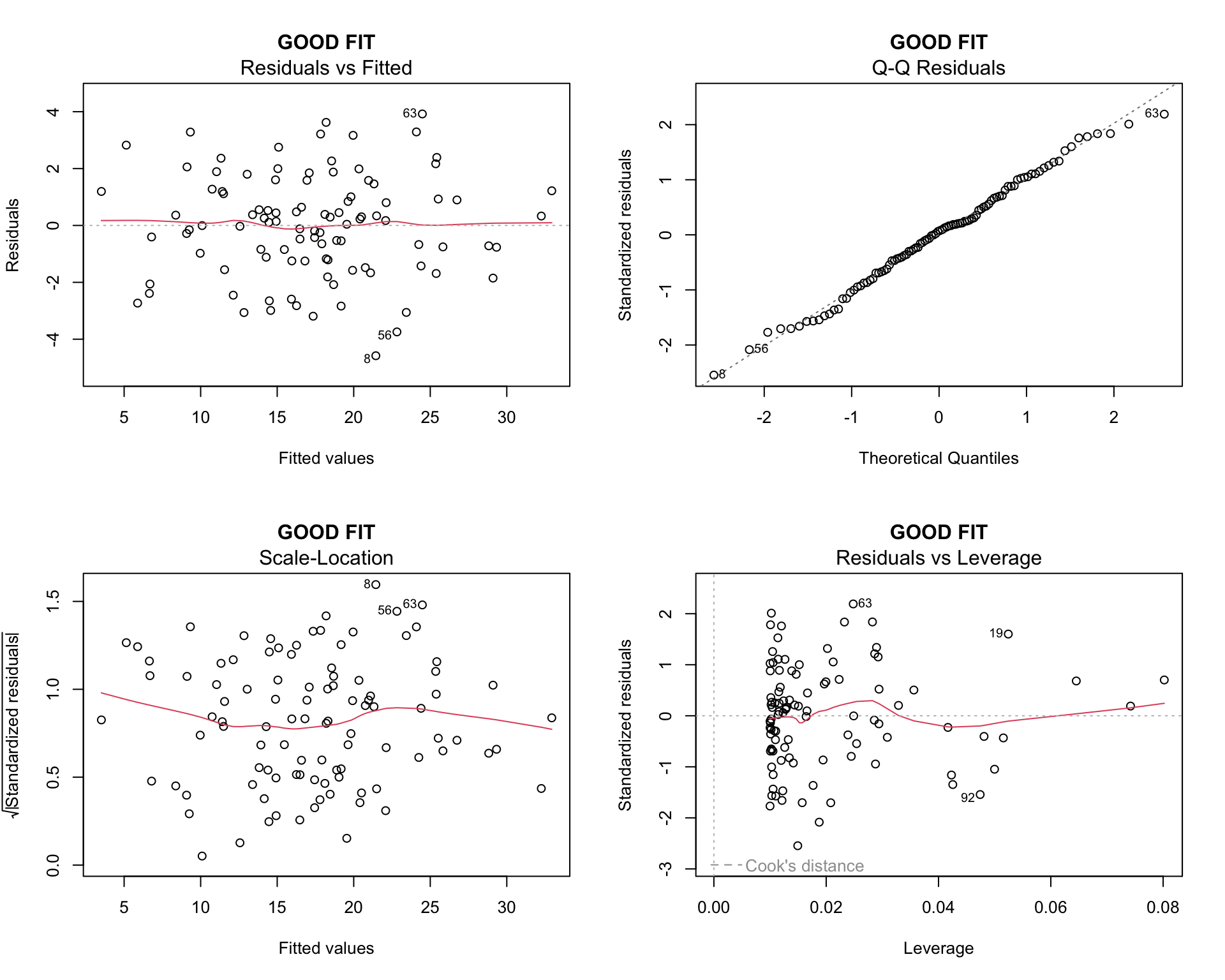
par(mfrow = c(1, 1))Interpretation:
- Residuals vs Fitted: Random scatter around zero, no pattern
- Q-Q plot: Points follow the line closely
- Scale-Location: Horizontal line with random scatter
- Residuals vs Leverage: No points with high leverage and high residuals
Bad fit: Non-linear relationship
When the true relationship is quadratic but we fit a linear model:
# Induce quadratic relationship
x2 <- seq(-3, 3, length.out = n)
# Quadratic
y2 <- 2 + 3 * x2 + 2 * x2^2 + rnorm(n, mean = 0, sd = 3)
model2 <- lm(y2 ~ x2)

par(mfrow = c(2, 2))
plot(model2, main = "BAD: Non-linear")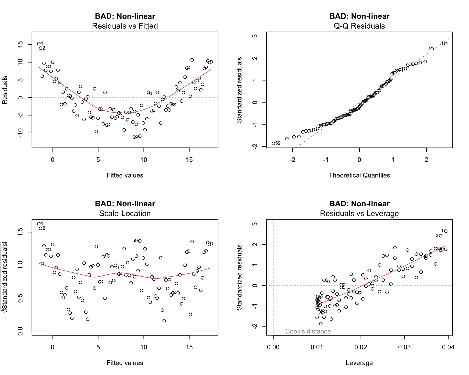
par(mfrow = c(1, 1))Issues:
- Residuals vs Fitted: Clear U-shaped pattern indicating non-linearity
- Q-Q plot: Deviation from the line at the tails
Bad fit: Heteroscedasticity
When variance of residuals increases with X:
# Inject variance
x3 <- runif(n, 0, 10)
# Variance increases with x
y3 <- 2 + 3 * x3 + rnorm(n, mean = 0, sd = x3)
model3 <- lm(y3 ~ x3)

par(mfrow = c(2, 2))
plot(model3, main = "BAD: Heteroscedasticity")
par(mfrow = c(1, 1))Issues:
- Residuals vs Fitted: Funnel-shaped pattern (variance increases)
- Scale-Location: Upward trend indicating non-constant variance
Bad fit: Non-normal residuals
When residuals don’t follow a normal distribution:
# Residuals are non-normal
x4 <- rnorm(n, mean = 5, sd = 2)
# Exponential errors
y4 <- 2 + 3 * x4 + rexp(n, rate = 0.5)
model4 <- lm(y4 ~ x4)

par(mfrow = c(2, 2))
plot(model4, main = "BAD: Non-normal residuals")
par(mfrow = c(1, 1))Issues:
- Q-Q plot: Strong deviation from the line, especially at the upper tail
- Residuals vs fitted: May show some asymmetry
Bad Fit: Influential outliers
When a few points have high leverage and high residuals:
# Outliers
x5 <- rnorm(n, mean = 5, sd = 2)
y5 <- 2 + 3 * x5 + rnorm(n, mean = 0, sd = 2)
# Add influential outliers
x5[1:3] <- c(15, 16, 17)
y5[1:3] <- c(10, 12, 8)
model5 <- lm(y5 ~ x5)

par(mfrow = c(2, 2))
plot(model5, main = "BAD: Influential outliers")
par(mfrow = c(1, 1))Issues:
- Residuals vs Leverage: Points labeled (1, 2, 3) in the bottom right region (high Cook’s distance)
- Residuals vs Fitted: These points stand out as unusual
Summary
When fitting linear models, always check diagnostic plots:
- Residuals vs Fitted: Look for random scatter (no patterns)
- Q-Q plot: Points should follow the line
- Scale-Location: Should be roughly horizontal
- Residuals vs Leverage: Watch for high-influence points
If these assumptions are violated, consider:
- Transforming variables
- Using non-linear models
- Removing or investigating outliers
- Using robust regression methods