---
title: "Ridge vs Lasso"
---
## Introduction
This notebook provides mathematical derivations for ridge and lasso regression.
## Setup
```{r setup}
#| label: setup
library(tidyverse)
library(glmnet)
library(MASS)
library(patchwork)
library(ggpubr)
theme_set(theme_minimal(base_size = 12))
```
# OLS
We have data: $(x_i, y_i)$ for $i = 1, \ldots, n$, where each $x_i = (x_{i1}, x_{i2}, \ldots, x_{ip})$ is a vector of $p$ predictors.
The linear model predicts:
$$
\hat{y}_i = \beta_0 + \beta_1 x_{i1} + \beta_2 x_{i2} + \cdots + \beta_p x_{ip} = \beta_0 + \sum_{j=1}^{p} \beta_j x_{ij}
$$
To keep things simple (and without loss of generality WLOG), we'll assume the predictors are **centered** (mean = 0), so we can drop the intercept $\beta_0$.
## Objective function
Minimize the **residual sum of squares (RSS)**:
$$
\text{RSS}(\beta) = \sum_{i=1}^{n} (y_i - \hat{y}_i)^2 = \sum_{i=1}^{n} \left(y_i - \sum_{j=1}^{p} \beta_j x_{ij}\right)^2
$$
To find the minimum, take the partial derivative with respect to each coefficient $\beta_k$ and set to zero.
$$
\text{RSS}(\beta) = \sum_{i=1}^{n} \left(y_i - \sum_{j=1}^{p} \beta_j x_{ij}\right)^2
$$
Using the chain rule:
$$
\frac{\partial \text{RSS}}{\partial \beta_k} = \frac{\partial}{\partial \beta_k} \sum_{i=1}^{n} \left(y_i - \sum_{j=1}^{p} \beta_j x_{ij}\right)^2
$$
$$
= \sum_{i=1}^{n} 2\left(y_i - \sum_{j=1}^{p} \beta_j x_{ij}\right) \cdot \frac{\partial}{\partial \beta_k}\left(y_i - \sum_{j=1}^{p} \beta_j x_{ij}\right)
$$
Note that:
$$
\frac{\partial}{\partial \beta_k}\left(y_i - \sum_{j=1}^{p} \beta_j x_{ij}\right) = \frac{\partial}{\partial \beta_k}(y_i - \beta_1 x_{i1} - \cdots - \beta_k x_{ik} - \cdots - \beta_p x_{ip})
$$
Only the term with $\beta_k$ matters:
$$
= -x_{ik}
$$
Therefore:
$$
\frac{\partial \text{RSS}}{\partial \beta_k} = \sum_{i=1}^{n} 2\left(y_i - \sum_{j=1}^{p} \beta_j x_{ij}\right) \cdot (-x_{ik})
$$
$$
= -2 \sum_{i=1}^{n} x_{ik} \left(y_i - \sum_{j=1}^{p} \beta_j x_{ij}\right)
$$
Setting differential to zeor:
$$
-2 \sum_{i=1}^{n} x_{ik} \left(y_i - \sum_{j=1}^{p} \beta_j x_{ij}\right) = 0
$$
Divide by $-2$:
$$
\sum_{i=1}^{n} x_{ik} \left(y_i - \sum_{j=1}^{p} \beta_j x_{ij}\right) = 0
$$
Expand:
$$
\sum_{i=1}^{n} x_{ik} y_i - \sum_{i=1}^{n} x_{ik} \sum_{j=1}^{p} \beta_j x_{ij} = 0
$$
$$
\sum_{i=1}^{n} x_{ik} y_i = \sum_{i=1}^{n} x_{ik} \sum_{j=1}^{p} \beta_j x_{ij}
$$
$$
\sum_{i=1}^{n} x_{ik} y_i = \sum_{j=1}^{p} \beta_j \sum_{i=1}^{n} x_{ik} x_{ij}
$$
The 'Normal' equation: This gives us $p$ equations (one for each $k = 1, \ldots, p$):
$$
\boxed{\sum_{j=1}^{p} \left(\sum_{i=1}^{n} x_{ik} x_{ij}\right) \beta_j = \sum_{i=1}^{n} x_{ik} y_i \quad \text{for } k = 1, \ldots, p}
$$
Alternatively, if this were to be written in **matrix form**, this is exactly:
$$
X^TX\beta = X^Ty
$$
where:
- $(X^TX)_{kj} = \sum_{i=1}^{n} x_{ik} x_{ij}$ (the $(k,j)$ entry of the matrix $X^TX$)
- $(X^Ty)_k = \sum_{i=1}^{n} x_{ik} y_i$ (the $k$-th entry of the vector $X^Ty$)
**Solution**:
$$
\hat{\beta}^{\text{OLS}} = (X^TX)^{-1}X^Ty
$$
provided $(X^TX)$ is invertible.
## Why is 'OLS' ordinary?
It is the 'vanilla' model that often serves as a baseline. However, it has some issues:
1. **Multicollinearity**: If predictors are correlated, $X^TX$ is nearly singular → $(X^TX)^{-1}$ is unstable
2. **High variance**: Small changes in data cause large changes in $\hat{\beta}$
3. **$p > n$ problem**: If more predictors than observations, $X^TX$ is not invertible
# Ridge regression
## Objective function
Ridge adds a **penalty** on the squared coefficients:
$$
L(\beta) = \sum_{i=1}^{n} \left(y_i - \sum_{j=1}^{p} \beta_j x_{ij}\right)^2 + \lambda \sum_{j=1}^{p} \beta_j^2
$$
where $\lambda \geq 0$ is the **regularization parameter**.
**Intuition**: The penalty $\lambda \sum_{j=1}^{p} \beta_j^2$ discourages large coefficients, reducing variance.
$$
L(\beta) = \underbrace{\sum_{i=1}^{n} \left(y_i - \sum_{j=1}^{p} \beta_j x_{ij}\right)^2}_{\text{RSS: fit to data}} + \underbrace{\lambda \sum_{j=1}^{p} \beta_j^2}_{\text{Penalty: keep coefficients small}}
$$
First term (RSS):
$$
\frac{\partial}{\partial \beta_k} \sum_{i=1}^{n} \left(y_i - \sum_{j=1}^{p} \beta_j x_{ij}\right)^2 = -2 \sum_{i=1}^{n} x_{ik} \left(y_i - \sum_{j=1}^{p} \beta_j x_{ij}\right)
$$
Same as OLS.
Second term (penalty):
$$
\frac{\partial}{\partial \beta_k} \lambda \sum_{j=1}^{p} \beta_j^2 = \lambda \cdot 2\beta_k = 2\lambda \beta_k
$$
(Only the $\beta_k^2$ term contributes to the derivative with respect to $\beta_k$)
**Total derivative**:
$$
\frac{\partial L}{\partial \beta_k} = -2 \sum_{i=1}^{n} x_{ik} \left(y_i - \sum_{j=1}^{p} \beta_j x_{ij}\right) + 2\lambda \beta_k
$$
Equating to zero:
$$
-2 \sum_{i=1}^{n} x_{ik} \left(y_i - \sum_{j=1}^{p} \beta_j x_{ij}\right) + 2\lambda \beta_k = 0
$$
Divide by $2$:
$$
-\sum_{i=1}^{n} x_{ik} \left(y_i - \sum_{j=1}^{p} \beta_j x_{ij}\right) + \lambda \beta_k = 0
$$
Rearrange:
$$
\sum_{i=1}^{n} x_{ik} \left(y_i - \sum_{j=1}^{p} \beta_j x_{ij}\right) = \lambda \beta_k
$$
Expand the left side:
$$
\sum_{i=1}^{n} x_{ik} y_i - \sum_{i=1}^{n} x_{ik} \sum_{j=1}^{p} \beta_j x_{ij} = \lambda \beta_k
$$
$$
\sum_{i=1}^{n} x_{ik} y_i - \sum_{j=1}^{p} \beta_j \sum_{i=1}^{n} x_{ik} x_{ij} = \lambda \beta_k
$$
Move the $\lambda \beta_k$ term to the left:
$$
\sum_{j=1}^{p} \beta_j \sum_{i=1}^{n} x_{ik} x_{ij} + \lambda \beta_k = \sum_{i=1}^{n} x_{ik} y_i
$$
The 'normal' equations:
For $k = 1, \ldots, p$:
$$
\sum_{j=1}^{p} \beta_j \sum_{i=1}^{n} x_{ik} x_{ij} + \lambda \beta_k = \sum_{i=1}^{n} x_{ik} y_i
$$
When $j = k$, the term $\sum_{i=1}^{n} x_{ik} x_{ik} = \sum_{i=1}^{n} x_{ik}^2$ gets an extra $+\lambda$ added to it.
In matrix notation, this becomes:
$$
(X^TX + \lambda I)\beta = X^Ty
$$
where $I$ is the identity matrix. The diagonal terms of $X^TX$ get $\lambda$ added to them.
**Solution**:
$$
\boxed{\hat{\beta}^{\text{Ridge}} = (X^TX + \lambda I)^{-1}X^Ty}
$$
## Why does this work?
Always invertible (even if $X^TX$ is not): Even if $X^TX$ is singular (not invertible), adding $\lambda I$ ensures:
$$
X^TX + \lambda I \text{ is always invertible when } \lambda > 0
$$
The eigenvalues of $X^TX + \lambda I$ are $(\text{eigenvalue of } X^TX) + \lambda$, which are always positive when $\lambda > 0$.
As $\lambda$ increases:
- **Small $\lambda$**: Solution close to OLS
- **Large $\lambda$**: Coefficients shrink toward zero
- **$\lambda \to \infty$**: $\hat{\beta}^{\text{Ridge}} \to 0$
Let's see this mathematically. Rewrite the normal equations:
$$
\sum_{j=1}^{p} \beta_j \sum_{i=1}^{n} x_{ik} x_{ij} = \sum_{i=1}^{n} x_{ik} y_i - \lambda \beta_k
$$
The right side is reduced by $\lambda \beta_k$, which "shrinks" the solution.
### Bias-Variance tradeoff
- **OLS**: Unbiased ($E[\hat{\beta}^{\text{OLS}}] = \beta^{\text{true}}$) but **high variance**
- **Ridge**: Biased ($E[\hat{\beta}^{\text{Ridge}}] \neq \beta^{\text{true}}$) but **lower variance**
- **Optimal $\lambda$**: Minimizes total MSE = Bias² + Variance
# Lasso regression
## Objective Function
Least absolute shrinkage and selection operator (Lasso) uses an **L1 penalty** (absolute values instead of squares):
$$
L(\beta) = \sum_{i=1}^{n} \left(y_i - \sum_{j=1}^{p} \beta_j x_{ij}\right)^2 + \lambda \sum_{j=1}^{p} |\beta_j|
$$
It does not have a closed-form solution like OLS or Ridge.
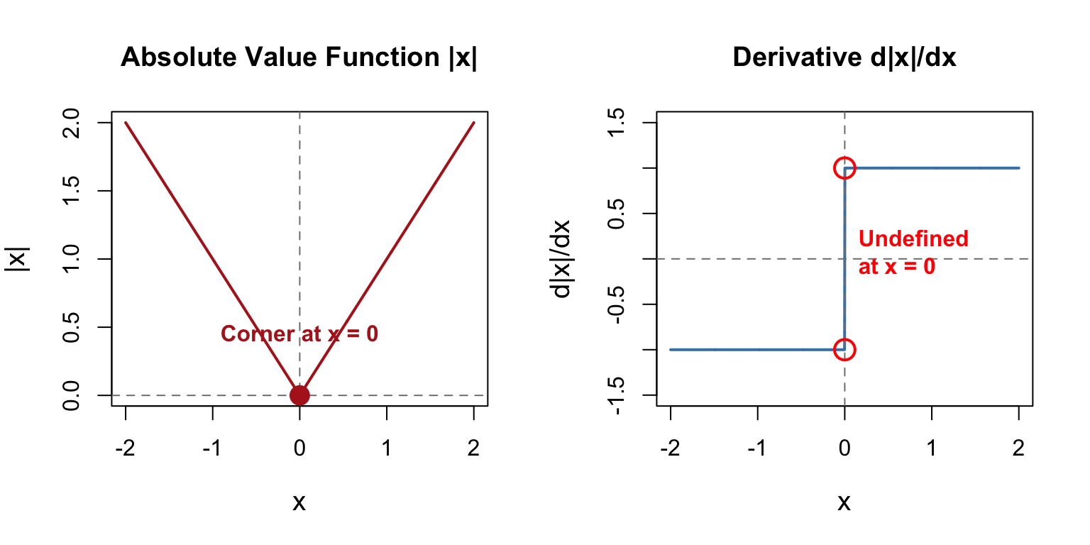
The absolute value function $|\beta_k|$ is **not differentiable** at $\beta_k = 0$.
**Derivative of $|\beta_k|$**:
$$
\frac{d |\beta_k|}{d \beta_k} = \begin{cases}
+1 & \text{if } \beta_k > 0 \\
-1 & \text{if } \beta_k < 0 \\
\text{undefined} & \text{if } \beta_k = 0
\end{cases}
$$
**Graphically**:
```{r abs-plot}
#| label: fig-abs-derivative
#| fig-cap: "The absolute value function has a corner at zero, making it non-differentiable"
#| fig-width: 8
#| fig-height: 4
par(mfrow = c(1, 2))

# Plot |x|
x <- seq(-2, 2, length.out = 1000)
plot(x, abs(x), type = "l", lwd = 2, col = "firebrick",
     main = "Absolute Value Function |x|",
     xlab = "x", ylab = "|x|", cex.lab = 1.2)
abline(v = 0, lty = 2, col = "gray50")
abline(h = 0, lty = 2, col = "gray50")
points(0, 0, pch = 16, cex = 2, col = "firebrick")
text(0, 0.3, "Corner at x = 0", pos = 3, col = "firebrick", font = 2)

# Plot derivative
x <- seq(-2, 2, length.out = 1000)
deriv <- ifelse(x > 0, 1, ifelse(x < 0, -1, NA))
plot(x, deriv, type = "l", lwd = 2, col = "steelblue",
     main = "Derivative d|x|/dx",
     xlab = "x", ylab = "d|x|/dx", ylim = c(-1.5, 1.5), cex.lab = 1.2)
abline(v = 0, lty = 2, col = "gray50")
abline(h = 0, lty = 2, col = "gray50")
points(0, 1, pch = 1, cex = 2, col = "red", lwd = 2)
points(0, -1, pch = 1, cex = 2, col = "red", lwd = 2)
text(0, 0, "Undefined\nat x = 0", pos = 4, col = "red", font = 2)

par(mfrow = c(1, 1))
```
### The Subgradient
At $\beta_k = 0$, we use the **subgradient**:
$$
\partial |\beta_k| = \begin{cases}
\{+1\} & \text{if } \beta_k > 0 \\
\{-1\} & \text{if } \beta_k < 0 \\
[-1, +1] & \text{if } \beta_k = 0
\end{cases}
$$
When $\beta_k = 0$, the subgradient is the **interval** $[-1, +1]$. This means there's no unique "slope" at zero.
## Solving Lasso: The two cases
Let's work through what happens when we try to solve for a single coefficient $\beta_k$, holding all others fixed.
For simplicity, assume we have **orthonormal** predictors (scaled so $\sum_{i=1}^{n} x_{ik}^2 = 1$ and predictors are uncorrelated). This simplifies the math without losing the key insight.
The objective for coefficient $\beta_k$ (with others fixed) becomes:
$$
L(\beta_k) = \sum_{i=1}^{n} \left(y_i - \sum_{j \neq k} \beta_j x_{ij} - \beta_k x_{ik}\right)^2 + \lambda |\beta_k|
$$
Let $r_k^{(i)} = y_i - \sum_{j \neq k} \beta_j x_{ij}$ be the **partial residual** (what's left after removing the effect of all other predictors).
Then:
$$
L(\beta_k) = \sum_{i=1}^{n} (r_k^{(i)} - \beta_k x_{ik})^2 + \lambda |\beta_k|
$$
Expand the squared term:
$$
L(\beta_k) = \sum_{i=1}^{n} [(r_k^{(i)})^2 - 2r_k^{(i)} \beta_k x_{ik} + \beta_k^2 x_{ik}^2] + \lambda |\beta_k|
$$
The first term $\sum (r_k^{(i)})^2$ doesn't depend on $\beta_k$, so we can drop it:
$$
L(\beta_k) = -2\beta_k \sum_{i=1}^{n} r_k^{(i)} x_{ik} + \beta_k^2 \sum_{i=1}^{n} x_{ik}^2 + \lambda |\beta_k|
$$
With orthonormal predictors, $\sum_{i=1}^{n} x_{ik}^2 = 1$. Let $z_k = \sum_{i=1}^{n} r_k^{(i)} x_{ik}$ (correlation between partial residual and predictor).
**Simplified objective**:
$$
L(\beta_k) = -2\beta_k z_k + \beta_k^2 + \lambda |\beta_k|
$$
Now let's solve this in **two cases**.
---
### Case 1: When $\beta_k > 0$
When $\beta_k > 0$, we have $|\beta_k| = \beta_k$, so:
$$
L(\beta_k) = -2\beta_k z_k + \beta_k^2 + \lambda \beta_k
$$
Take the derivative:
$$
\frac{dL}{d\beta_k} = -2z_k + 2\beta_k + \lambda
$$
Set equal to zero:
$$
-2z_k + 2\beta_k + \lambda = 0
$$
Solve for $\beta_k$:
$$
\beta_k = z_k - \frac{\lambda}{2}
$$
But this is only valid if $\beta_k > 0$, which requires:
$$
z_k - \frac{\lambda}{2} > 0 \quad \Rightarrow \quad z_k > \frac{\lambda}{2}
$$
**Lasso solution when $\beta_k > 0$**:
$$
\boxed{\hat{\beta}_k^{\text{Lasso}} = z_k - \frac{\lambda}{2} \quad \text{if } z_k > \frac{\lambda}{2}}
$$
---
### Case 2: When $\beta_k < 0$
When $\beta_k < 0$, we have $|\beta_k| = -\beta_k$, so:
$$
L(\beta_k) = -2\beta_k z_k + \beta_k^2 - \lambda \beta_k
$$
Take the derivative:
$$
\frac{dL}{d\beta_k} = -2z_k + 2\beta_k - \lambda
$$
Set equal to zero:
$$
-2z_k + 2\beta_k - \lambda = 0
$$
Solve for $\beta_k$:
$$
\beta_k = z_k + \frac{\lambda}{2}
$$
This is only valid if $\beta_k < 0$, which requires:
$$
z_k + \frac{\lambda}{2} < 0 \quad \Rightarrow \quad z_k < -\frac{\lambda}{2}
$$
**Lasso solution when $\beta_k < 0$**:
$$
\boxed{\hat{\beta}_k^{\text{Lasso}} = z_k + \frac{\lambda}{2} \quad \text{if } z_k < -\frac{\lambda}{2}}
$$
---
### Case 3: When $|z_k| \leq \frac{\lambda}{2}$
If $-\frac{\lambda}{2} \leq z_k \leq \frac{\lambda}{2}$:
- Assuming $\beta_k > 0$ gives $\beta_k = z_k - \frac{\lambda}{2} < 0$ (contradiction!)
- Assuming $\beta_k < 0$ gives $\beta_k = z_k + \frac{\lambda}{2} > 0$ (contradiction!)
The only consistent solution is:
$$
\boxed{\hat{\beta}_k^{\text{Lasso}} = 0 \quad \text{if } |z_k| \leq \frac{\lambda}{2}}
$$
This is the **shrinkage to zero**!
---
### Complete Lasso Solution
Combining all three cases:
$$
\boxed{\hat{\beta}_k^{\text{Lasso}} = \begin{cases}
z_k - \frac{\lambda}{2} & \text{if } z_k > \frac{\lambda}{2} \\
0 & \text{if } |z_k| \leq \frac{\lambda}{2} \\
z_k + \frac{\lambda}{2} & \text{if } z_k < -\frac{\lambda}{2}
\end{cases}}
$$
This is exactly the **soft-thresholding operator**:
$$
\hat{\beta}_k^{\text{Lasso}} = S\left(z_k, \frac{\lambda}{2}\right) = \text{sign}(z_k) \left(|z_k| - \frac{\lambda}{2}\right)_+
$$
where $(a)_+ = \max(a, 0)$.
---
## Ridge vs Lasso
Now let's compare with **Ridge regression** for the same setup.
### Ridge solution
For Ridge, the objective is:
$$
L(\beta_k) = -2\beta_k z_k + \beta_k^2 + \lambda \beta_k^2 = -2\beta_k z_k + (1+\lambda)\beta_k^2
$$
Take the derivative (always well-defined since $\beta_k^2$ is smooth):
$$
\frac{dL}{d\beta_k} = -2z_k + 2(1+\lambda)\beta_k = 0
$$
Solve:
$$
\boxed{\hat{\beta}_k^{\text{Ridge}} = \frac{z_k}{1+\lambda}}
$$
Ridge solution is **always proportional** to $z_k$. If $z_k \neq 0$, then $\hat{\beta}_k^{\text{Ridge}} \neq 0$.
### Plot
```{r ridge-vs-lasso-shrinkage}
#| label: fig-ridge-lasso-shrinkage
#| fig-cap: "Ridge vs Lasso shrinkage: Ridge shrinks continuously, Lasso has a dead zone"
#| fig-width: 12
#| fig-height: 5
# Range of z values
z <- seq(-3, 3, length.out = 1000)
lambda <- 1

# Ridge solution
beta_ridge <- z / (1 + lambda)

# Lasso solution (soft-thresholding)
beta_lasso <- ifelse(z > lambda/2, z - lambda/2,
                     ifelse(z < -lambda/2, z + lambda/2, 0))

# Plot
par(mfrow = c(1, 2))

# Ridge
plot(z, beta_ridge, type = "l", lwd = 3, col = "steelblue",
     main = "Ridge: Continuous Shrinkage",
     xlab = expression(z[k] == sum(r[k]^(i) * x[ik], i==1, n)),
     ylab = expression(hat(beta)[k]),
     cex.lab = 1.2, cex.main = 1.3, ylim = c(-3, 3))
abline(h = 0, lty = 2, col = "gray50")
abline(v = 0, lty = 2, col = "gray50")
abline(a = 0, b = 1, lty = 3, col = "gray70", lwd = 2)  # OLS line
text(2, 2.5, "No exact zeros!", col = "steelblue", font = 2, cex = 1.2)
text(2, -2.5, expression(hat(beta)[k] == frac(z[k], 1+lambda)),
     col = "steelblue", font = 2, cex = 1.1)

# Lasso
plot(z, beta_lasso, type = "l", lwd = 3, col = "firebrick",
     main = "Lasso: Hard Thresholding",
     xlab = expression(z[k] == sum(r[k]^(i) * x[ik], i==1, n)),
     ylab = expression(hat(beta)[k]),
     cex.lab = 1.2, cex.main = 1.3, ylim = c(-3, 3))
abline(h = 0, lty = 2, col = "gray50")
abline(v = 0, lty = 2, col = "gray50")
abline(a = 0, b = 1, lty = 3, col = "gray70", lwd = 2)  # OLS line

# Highlight threshold region
rect(-lambda/2, -3, lambda/2, 3, col = rgb(1, 0, 0, 0.1), border = NA)
abline(v = c(-lambda/2, lambda/2), lty = 2, col = "firebrick", lwd = 1.5)

text(0, 2.5, "DEAD ZONE\nβ = 0", col = "firebrick", font = 2, cex = 1.2)
text(2, -2.5, expression(hat(beta)[k] == z[k] - frac(lambda, 2)),
     col = "firebrick", font = 2, cex = 1.1)

par(mfrow = c(1, 1))
```
| Property | Ridge | Lasso |
|----------|-------|-------|
| **Formula** | $\hat{\beta}_k = \frac{z_k}{1+\lambda}$ | $\hat{\beta}_k = \text{sign}(z_k)(|z_k| - \frac{\lambda}{2})_+$ |
| **Derivative** | Smooth everywhere | Non-differentiable at $\beta_k = 0$ |
| **When $z_k$ is small** | $\hat{\beta}_k \approx \frac{z_k}{1+\lambda} \neq 0$ | $\hat{\beta}_k = 0$ if $|z_k| < \frac{\lambda}{2}$ |
| **Shrinkage type** | Proportional (continuous) | Threshold (discontinuous) |
| **Dead zone** | None | Yes: $|z_k| \leq \frac{\lambda}{2}$ |
| **Sparsity** | Never produces exact zeros | Produces exact zeros |
**Ridge**: Even if a predictor has a tiny correlation with the residual ($z_k$ small), Ridge still gives it a small non-zero coefficient. All predictors contribute something.
**Lasso**: If $|z_k| < \frac{\lambda}{2}$, the predictor is deemed **not useful enough** and its coefficient is set to exactly zero. Only "strong" predictors survive.
### Example
Let's see a concrete example:
```{r numerical-example}
#| label: tbl-ridge-lasso-example
#| tbl-cap: "Numerical comparison: Ridge vs Lasso for different z values"
lambda <- 1.0

z_values <- c(-2, -0.8, -0.4, -0.2, 0, 0.2, 0.4, 0.8, 2)

ridge_coefs <- z_values / (1 + lambda)
lasso_coefs <- ifelse(z_values > lambda/2, z_values - lambda/2,
                      ifelse(z_values < -lambda/2, z_values + lambda/2, 0))

comparison_df <- data.frame(
  z_k = z_values,
  Ridge = round(ridge_coefs, 3),
  Lasso = round(lasso_coefs, 3),
  Difference = round(abs(ridge_coefs - lasso_coefs), 3)
)

knitr::kable(comparison_df,
             col.names = c("$z_k$", "Ridge: $\\frac{z_k}{1+\\lambda}$",
                          "Lasso: $S(z_k, \\frac{\\lambda}{2})$",
                          "|Difference|"),
             align = "c")
```
**Observation**: When $|z_k| \leq 0.5$, Lasso sets coefficient to **exactly zero**, while Ridge keeps small non-zero values.
---
## Solving Lasso: Coordinate descent
Since there's no closed-form solution, we use **iterative algorithms**. The most popular is **coordinate descent**:
**Algorithm**:
1. Initialize $\hat{\beta}^{(0)}$ (e.g., all zeros or OLS solution)
2. Repeat until convergence:
- For each $j = 1, \ldots, p$:
a. Compute **partial residual** (holding other coefficients fixed):
$$
r_j = y - \sum_{k \neq j} x_k \hat{\beta}_k
$$
b. Update $\hat{\beta}_j$ using **soft-thresholding**:
$$
\hat{\beta}_j \leftarrow \frac{S(x_j^T r_j, \lambda)}{\|x_j\|^2}
$$
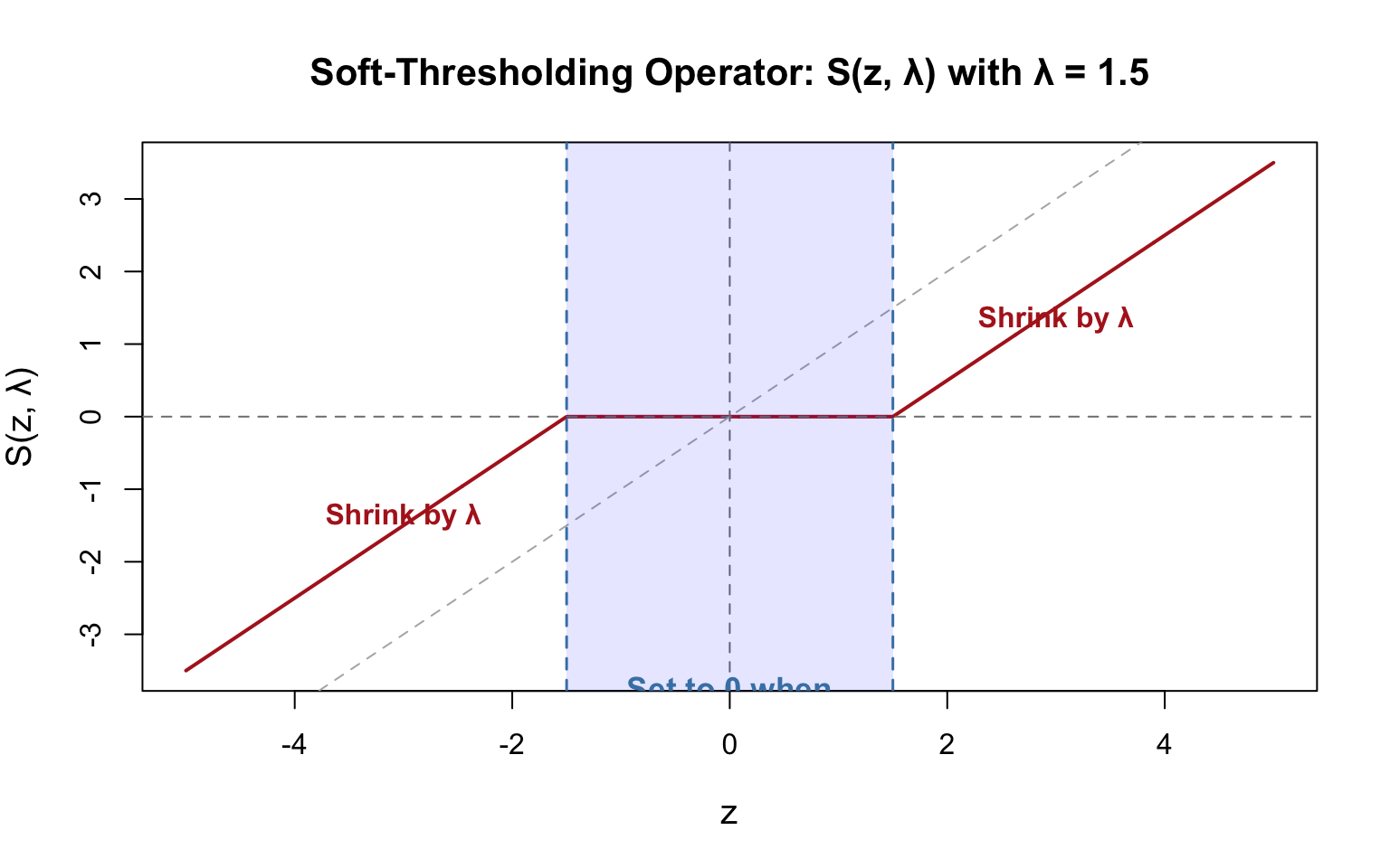
where the soft-thresholding operator is:
$$
S(z, \lambda) = \begin{cases}
z - \lambda & \text{if } z > \lambda \\
0 & \text{if } |z| \leq \lambda \\
z + \lambda & \text{if } z < -\lambda
\end{cases}
$$
3. Check convergence: Stop when coefficients don't change much
### Soft-thresholding operator
The soft-thresholding operator **automatically sets coefficients to zero** when $|x_j^T r_j| < \lambda$:
```{r soft-thresh}
#| label: fig-soft-thresh
#| fig-cap: "Soft-thresholding operator: sets values to zero when |z| < λ"
#| fig-width: 8
#| fig-height: 5
soft_threshold <- function(z, lambda) {
  ifelse(z > lambda, z - lambda,
         ifelse(z < -lambda, z + lambda, 0))
}

z <- seq(-5, 5, length.out = 1000)
lambda <- 1.5

plot(z, soft_threshold(z, lambda), type = "l", lwd = 2, col = "firebrick",
     main = paste("Soft-Thresholding Operator: S(z, λ) with λ =", lambda),
     xlab = "z", ylab = "S(z, λ)", cex.lab = 1.2, cex.main = 1.3)
abline(v = 0, lty = 2, col = "gray50")
abline(h = 0, lty = 2, col = "gray50")
abline(a = 0, b = 1, lty = 2, col = "gray70")  # y = z line for reference

# Highlight the threshold region
rect(-lambda, -6, lambda, 6, col = rgb(0, 0, 1, 0.1), border = NA)
abline(v = c(-lambda, lambda), lty = 2, col = "steelblue", lwd = 1.5)

text(0, -4, paste("Set to 0 when\n|z| <", lambda),
     col = "steelblue", font = 2, cex = 1.1)
text(3, 1, "Shrink by λ", pos = 3, col = "firebrick", font = 2)
text(-3, -1, "Shrink by λ", pos = 1, col = "firebrick", font = 2)
```
This is why Lasso produces **sparse solutions**: coefficients can be exactly zero!
## Ridge vs Lasso: Key Differences
| Aspect | Ridge | Lasso |
|--------|-------|-------|
| **Penalty term** | $\lambda \sum_{j=1}^{p} \beta_j^2$ | $\lambda \sum_{j=1}^{p} |\beta_j|$ |
| **Derivative of penalty** | $2\lambda \beta_j$ (always defined) | $\lambda \cdot \text{sign}(\beta_j)$ (undefined at 0) |
| **Solution method** | Closed-form: solve linear system | Iterative: coordinate descent |
| **Coefficient behavior** | Shrink toward zero (never exactly zero) | Can be exactly zero |
| **Normal equations** | $\sum_j \beta_j \sum_i x_{ik} x_{ij} + \lambda \beta_k = \sum_i x_{ik} y_i$ | No simple equation (subgradient) |
| **Variable selection** | No | Yes |
The soft-thresholding operator in coordinate descent sets $\hat{\beta}_j = 0$ when:
$$
\left|\sum_{i=1}^{n} x_{ij} r_j\right| < \lambda
$$
where $r_j$ is the partial residual.
**Intuition**: If the correlation between predictor $x_j$ and the partial residual is weak (less than $\lambda$), Lasso decides that predictor is not useful and sets its coefficient to zero.
**Ridge never does this**: Its update rule is:
$$
\hat{\beta}_j \leftarrow \frac{\sum_{i=1}^{n} x_{ij} r_j}{\sum_{i=1}^{n} x_{ij}^2 + \lambda}
$$
The denominator $\sum_{i=1}^{n} x_{ij}^2 + \lambda > 0$ always, so $\hat{\beta}_j$ can get very small but never exactly zero.
# Geometric Interpretation
The geometric interpretation is the same whether we use matrix or scalar notation. I'll include the key visualizations from the matrix version.
## Constraint regions
```{r constraint-regions-scalar}
#| label: fig-constraint-regions-scalar
#| fig-cap: "Ridge (circle) vs Lasso (diamond) constraint regions"
#| fig-width: 12
#| fig-height: 5
# Ridge: circle
theta <- seq(0, 2*pi, length.out = 1000)
ridge_constraint <- data.frame(
  beta1 = cos(theta),
  beta2 = sin(theta)
)

# Lasso: diamond
lasso_constraint <- data.frame(
  beta1 = c(1, 0, -1, 0, 1),
  beta2 = c(0, 1, 0, -1, 0)
)

p_ridge <- ggplot(ridge_constraint, aes(beta1, beta2)) +
  geom_polygon(fill = "steelblue", alpha = 0.3) +
  geom_path(color = "steelblue", linewidth = 1.5) +
  coord_fixed(xlim = c(-1.2, 1.2), ylim = c(-1.2, 1.2)) +
  geom_hline(yintercept = 0, linetype = "dashed", alpha = 0.5) +
  geom_vline(xintercept = 0, linetype = "dashed", alpha = 0.5) +
  labs(title = "Ridge: Smooth Circle",
       subtitle = expression(sum(beta[j]^2, j==1, p) <= t),
       x = expression(beta[1]), y = expression(beta[2])) +
  theme_minimal(base_size = 12)

p_lasso <- ggplot(lasso_constraint, aes(beta1, beta2)) +
  geom_polygon(fill = "firebrick", alpha = 0.3) +
  geom_path(color = "firebrick", linewidth = 1.5) +
  coord_fixed(xlim = c(-1.2, 1.2), ylim = c(-1.2, 1.2)) +
  geom_hline(yintercept = 0, linetype = "dashed", alpha = 0.5) +
  geom_vline(xintercept = 0, linetype = "dashed", alpha = 0.5) +
  labs(title = "Lasso: Diamond with Corners",
       subtitle = expression(sum("|"*beta[j]*"|", j==1, p) <= t),
       x = expression(beta[1]), y = expression(beta[2])) +
  theme_minimal(base_size = 12)

p_ridge + p_lasso
```
Lasso's diamond has corners on the axes → RSS contours likely touch at a corner → some $\beta_j = 0$.
## Contours
```{r practical-example-scalar}
#| label: practical-example-scalar
set.seed(42)
n <- 50
X <- matrix(rnorm(n * 2), ncol = 2)
true_beta <- c(0.8, 0.6)
y <- X %*% true_beta + rnorm(n, sd = 0.5)

# OLS
beta_ols <- solve(t(X) %*% X) %*% t(X) %*% y

lambda_ridge <- 2
beta_ridge <- solve(t(X) %*% X + lambda_ridge * diag(2)) %*% t(X) %*% y

lasso_fit <- glmnet(X, y, alpha = 1, lambda = 0.5, standardize = FALSE)
beta_lasso <- as.vector(coef(lasso_fit))[-1]

rss <- function(beta1, beta2, X, y) {
  beta <- c(beta1, beta2)
  residuals <- y - X %*% beta
  sum(residuals^2)
}

beta1_seq <- seq(-0.2, 1.2, length.out = 200)
beta2_seq <- seq(-0.2, 1.2, length.out = 200)
grid <- expand.grid(beta1 = beta1_seq, beta2 = beta2_seq)
grid$rss <- mapply(rss, grid$beta1, grid$beta2, MoreArgs = list(X = X, y = y))

t_ridge <- sqrt(sum(beta_ridge^2))
ridge_scaled <- data.frame(
  beta1 = ridge_constraint$beta1 * t_ridge,
  beta2 = ridge_constraint$beta2 * t_ridge
)

t_lasso <- sum(abs(beta_lasso))
lasso_scaled <- data.frame(
  beta1 = lasso_constraint$beta1 * t_lasso,
  beta2 = lasso_constraint$beta2 * t_lasso
)
```
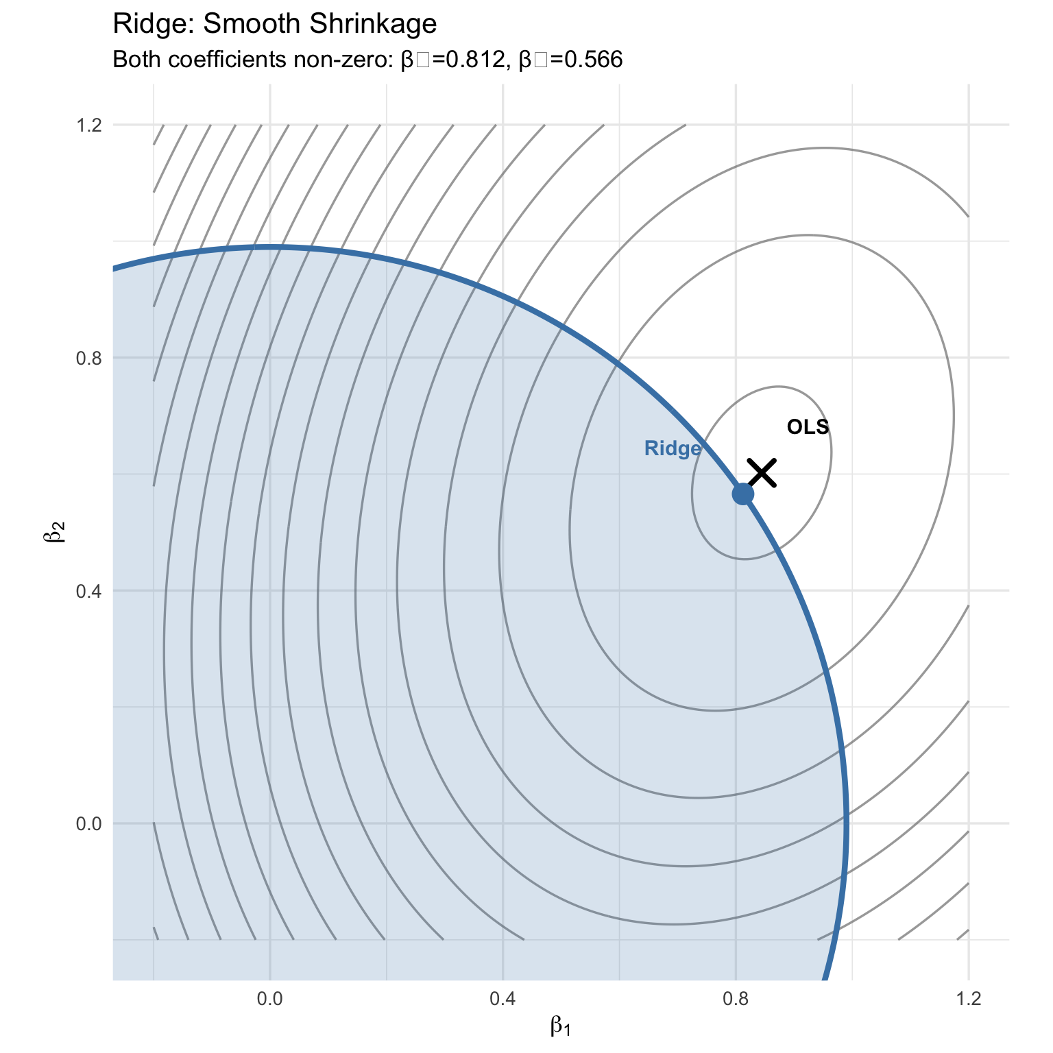
### Ridge with Contours
```{r ridge-geo-scalar}
#| label: fig-ridge-geo-scalar
#| fig-cap: "Ridge: Contours meet circle smoothly, no coefficients set to zero"
#| fig-width: 8
#| fig-height: 8
ggplot() +
  geom_contour(data = grid, aes(beta1, beta2, z = rss),
               bins = 20, color = "gray50", alpha = 0.7) +
  geom_polygon(data = ridge_scaled, aes(beta1, beta2),
               fill = "steelblue", alpha = 0.2) +
  geom_path(data = ridge_scaled, aes(beta1, beta2),
            color = "steelblue", linewidth = 1.5) +
  geom_point(aes(beta_ols[1], beta_ols[2]),
             color = "black", size = 5, shape = 4, stroke = 2) +
  geom_point(aes(beta_ridge[1], beta_ridge[2]),
             color = "steelblue", size = 5) +
  annotate("text", x = beta_ols[1] + 0.08, y = beta_ols[2] + 0.08,
           label = "OLS", fontface = "bold", size = 4) +
  annotate("text", x = beta_ridge[1] - 0.12, y = beta_ridge[2] + 0.08,
           label = "Ridge", color = "steelblue", fontface = "bold", size = 4) +
  coord_fixed(xlim = c(-0.2, 1.2), ylim = c(-0.2, 1.2)) +
  labs(title = "Ridge: Smooth Shrinkage",
       subtitle = sprintf("Both coefficients non-zero: β₁=%.3f, β₂=%.3f",
                          beta_ridge[1], beta_ridge[2]),
       x = expression(beta[1]), y = expression(beta[2])) +
  theme_minimal(base_size = 13)
```
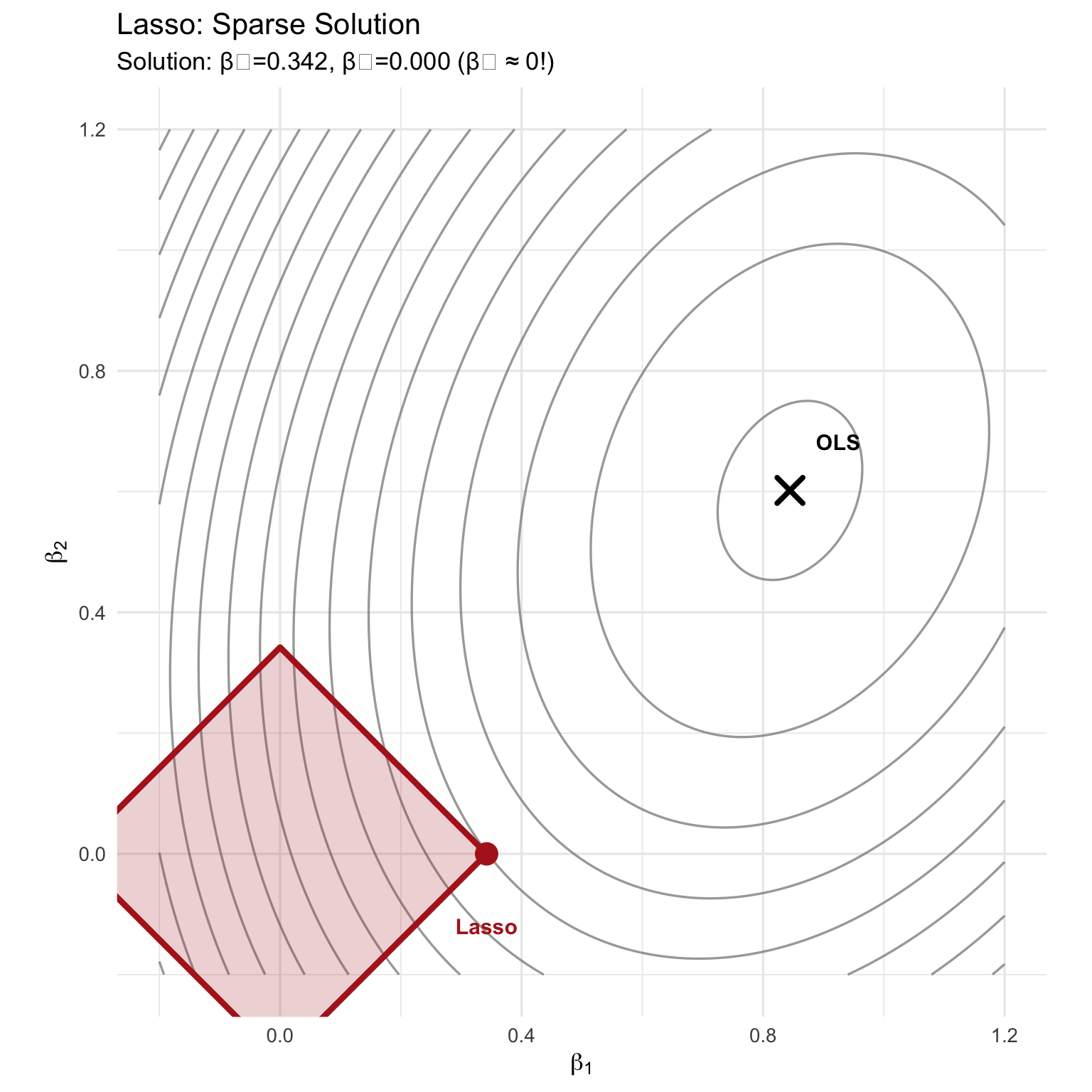
### Lasso with contours
```{r lasso-geo-scalar}
#| label: fig-lasso-geo-scalar
#| fig-cap: "Lasso: Contours often hit corners, producing sparse solutions"
#| fig-width: 8
#| fig-height: 8
ggplot() +
  geom_contour(data = grid, aes(beta1, beta2, z = rss),
               bins = 20, color = "gray50", alpha = 0.7) +
  geom_polygon(data = lasso_scaled, aes(beta1, beta2),
               fill = "firebrick", alpha = 0.2) +
  geom_path(data = lasso_scaled, aes(beta1, beta2),
            color = "firebrick", linewidth = 1.5) +
  geom_point(aes(beta_ols[1], beta_ols[2]),
             color = "black", size = 5, shape = 4, stroke = 2) +
  geom_point(aes(beta_lasso[1], beta_lasso[2]),
             color = "firebrick", size = 5) +
  annotate("text", x = beta_ols[1] + 0.08, y = beta_ols[2] + 0.08,
           label = "OLS", fontface = "bold", size = 4) +
  annotate("text", x = beta_lasso[1], y = beta_lasso[2] - 0.12,
           label = "Lasso", color = "firebrick", fontface = "bold", size = 4) +
  coord_fixed(xlim = c(-0.2, 1.2), ylim = c(-0.2, 1.2)) +
  labs(title = "Lasso: Sparse Solution",
       subtitle = sprintf("Solution: β₁=%.3f, β₂=%.3f %s",
                          beta_lasso[1], beta_lasso[2],
                          ifelse(abs(beta_lasso[2]) < 0.01, "(β₂ ≈ 0!)", "")),
       x = expression(beta[1]), y = expression(beta[2])) +
  theme_minimal(base_size = 13)
```
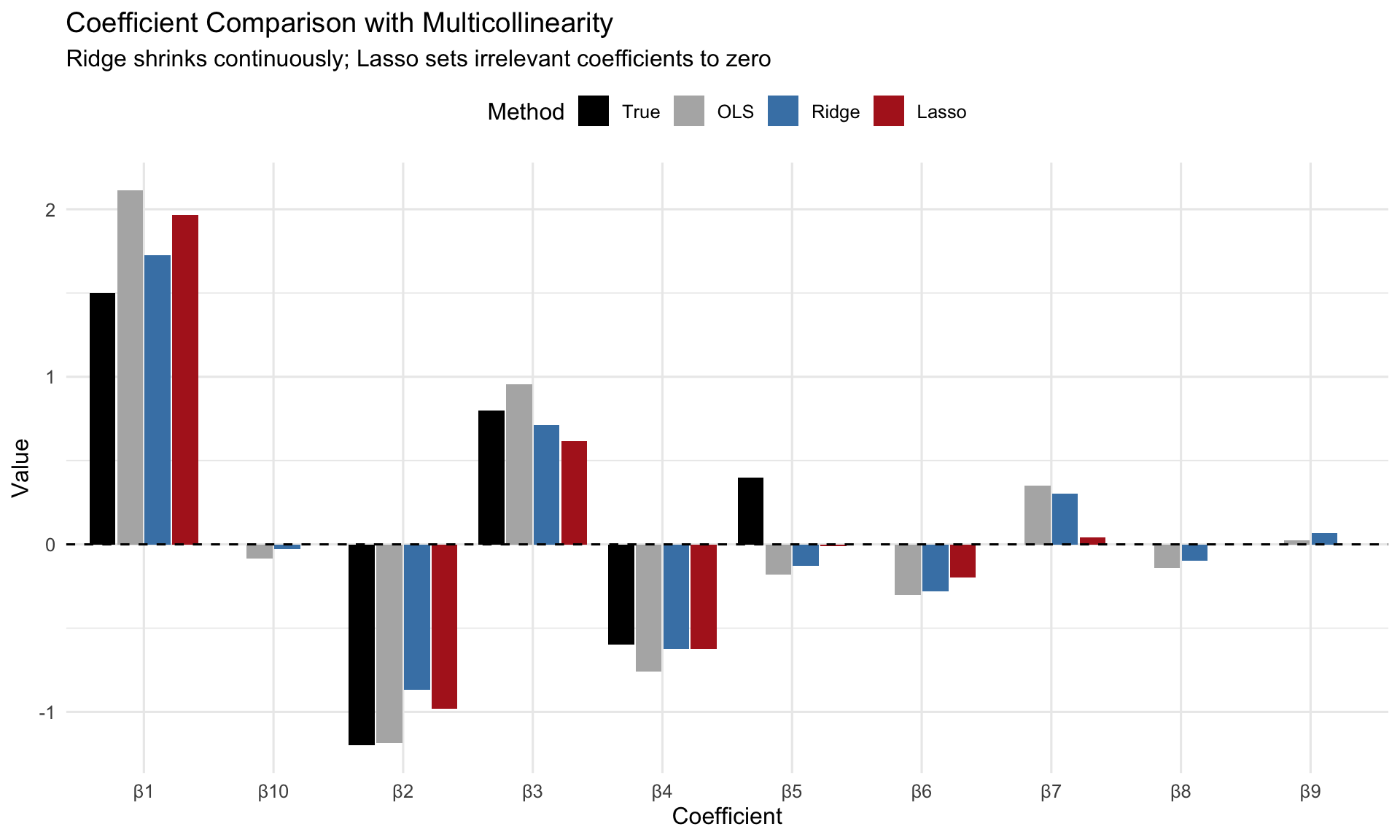
## Simulation: Multicollinearity
Let's compare Ridge and Lasso with correlated predictors.
```{r multicollinearity-sim}
#| label: multicollinearity-simulation
set.seed(123)
n <- 100
p <- 10

# Create correlation matrix (high multicollinearity)
rho <- 0.8
Sigma <- matrix(rho, p, p)
diag(Sigma) <- 1

# Generate predictors
X <- mvrnorm(n, mu = rep(0, p), Sigma = Sigma)

# True model: only first 5 predictors matter
true_beta <- c(1.5, -1.2, 0.8, -0.6, 0.4, rep(0, 5))
y <- X %*% true_beta + rnorm(n, sd = 1.5)

# Fit models
ridge_cv <- cv.glmnet(X, y, alpha = 0)
lasso_cv <- cv.glmnet(X, y, alpha = 1)

# Extract coefficients
ridge_coef <- as.vector(coef(ridge_cv, s = "lambda.min"))[-1]
lasso_coef <- as.vector(coef(lasso_cv, s = "lambda.min"))[-1]
ols_coef <- as.vector(coef(lm(y ~ X)))[-1]
```
### Coefficient Comparison
```{r coef-comparison}
#| label: fig-coef-comparison
#| fig-cap: "Coefficient estimates: OLS (unstable), Ridge (shrunk), Lasso (sparse)"
#| fig-width: 10
#| fig-height: 6
coef_df <- data.frame(
  Variable = rep(paste0("β", 1:p), 4),
  Value = c(true_beta, ols_coef, ridge_coef, lasso_coef),
  Method = rep(c("True", "OLS", "Ridge", "Lasso"), each = p)
) %>%
  mutate(Method = factor(Method, levels = c("True", "OLS", "Ridge", "Lasso")))

ggplot(coef_df, aes(x = Variable, y = Value, fill = Method)) +
  geom_col(position = position_dodge(width = 0.85), width = 0.8) +
  geom_hline(yintercept = 0, linetype = "dashed") +
  scale_fill_manual(values = c("True" = "black",
                                 "OLS" = "gray70",
                                 "Ridge" = "steelblue",
                                 "Lasso" = "firebrick")) +
  labs(title = "Coefficient Comparison with Multicollinearity",
       subtitle = "Ridge shrinks continuously; Lasso sets irrelevant coefficients to zero",
       x = "Coefficient", y = "Value") +
  theme_minimal(base_size = 12) +
  theme(legend.position = "top")
```
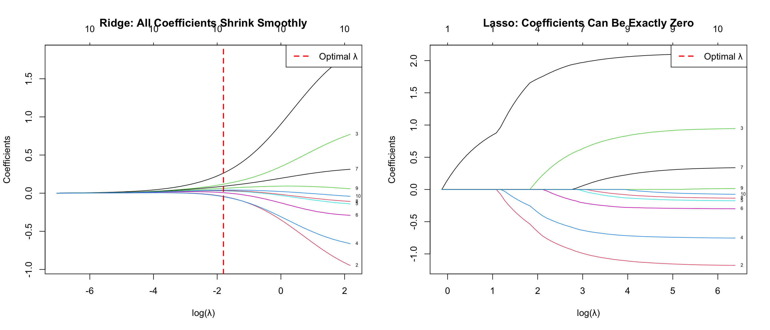
### Regularization Paths
```{r reg-paths}
#| label: fig-reg-paths
#| fig-cap: "Regularization paths: Ridge (left) never reaches zero; Lasso (right) produces exact zeros"
#| fig-width: 14
#| fig-height: 6
par(mfrow = c(1, 2))

# Ridge path
plot(ridge_cv$glmnet.fit, xvar = "lambda", label = TRUE,
     main = "Ridge: All Coefficients Shrink Smoothly",
     xlab = "log(λ)", ylab = "Coefficients")
abline(v = log(ridge_cv$lambda.min), lty = 2, col = "red", lwd = 2)
legend("topright", legend = "Optimal λ", lty = 2, col = "red", lwd = 2)

# Lasso path
plot(lasso_cv$glmnet.fit, xvar = "lambda", label = TRUE,
     main = "Lasso: Coefficients Can Be Exactly Zero",
     xlab = "log(λ)", ylab = "Coefficients")
abline(v = log(lasso_cv$lambda.min), lty = 2, col = "red", lwd = 2)
legend("topright", legend = "Optimal λ", lty = 2, col = "red", lwd = 2)

par(mfrow = c(1, 1))
```
### Sparsity comparison
```{r sparsity}
#| label: tbl-sparsity
#| tbl-cap: "Number of non-zero coefficients"
sparsity_df <- data.frame(
  Method = c("OLS", "Ridge", "Lasso"),
  Non_Zero_Coefficients = c(
    sum(ols_coef != 0),
    sum(abs(ridge_coef) > 1e-5),
    sum(abs(lasso_coef) > 1e-5)
  ),
  Exact_Zeros = c(
    sum(ols_coef == 0),
    sum(abs(ridge_coef) < 1e-10),
    sum(abs(lasso_coef) < 1e-10)
  )
)

knitr::kable(sparsity_df, col.names = c("Method", "Non-Zero", "Exact Zeros"))
```
## References
1. Hastie, T., Tibshirani, R., & Friedman, J. (2009). *The Elements of Statistical Learning* (2nd ed.). Springer. Chapter 3.
2. Tibshirani, R. (1996). "Regression Shrinkage and Selection via the Lasso". *Journal of the Royal Statistical Society: Series B*, 58(1), 267-288.
3. Friedman, J., Hastie, T., & Tibshirani, R. (2010). "Regularization Paths for Generalized Linear Models via Coordinate Descent". *Journal of Statistical Software*, 33(1), 1-22.