suppressPackageStartupMessages({

library(ggplot2)
library(gganimate)
library(dplyr)
library(tidyr)
library(gridExtra)
library(gifski)

})
theme_set(ggpubr::theme_pubr())
set.seed(42)PCA Animation
Simulate Data
x <- 1:100

error.x <- rnorm(n = 100, mean = 0, sd = 25)
error.y <- rnorm(n = 100, mean = 0, sd = 25)

y <- 25 + 2 * x
plot(x,y)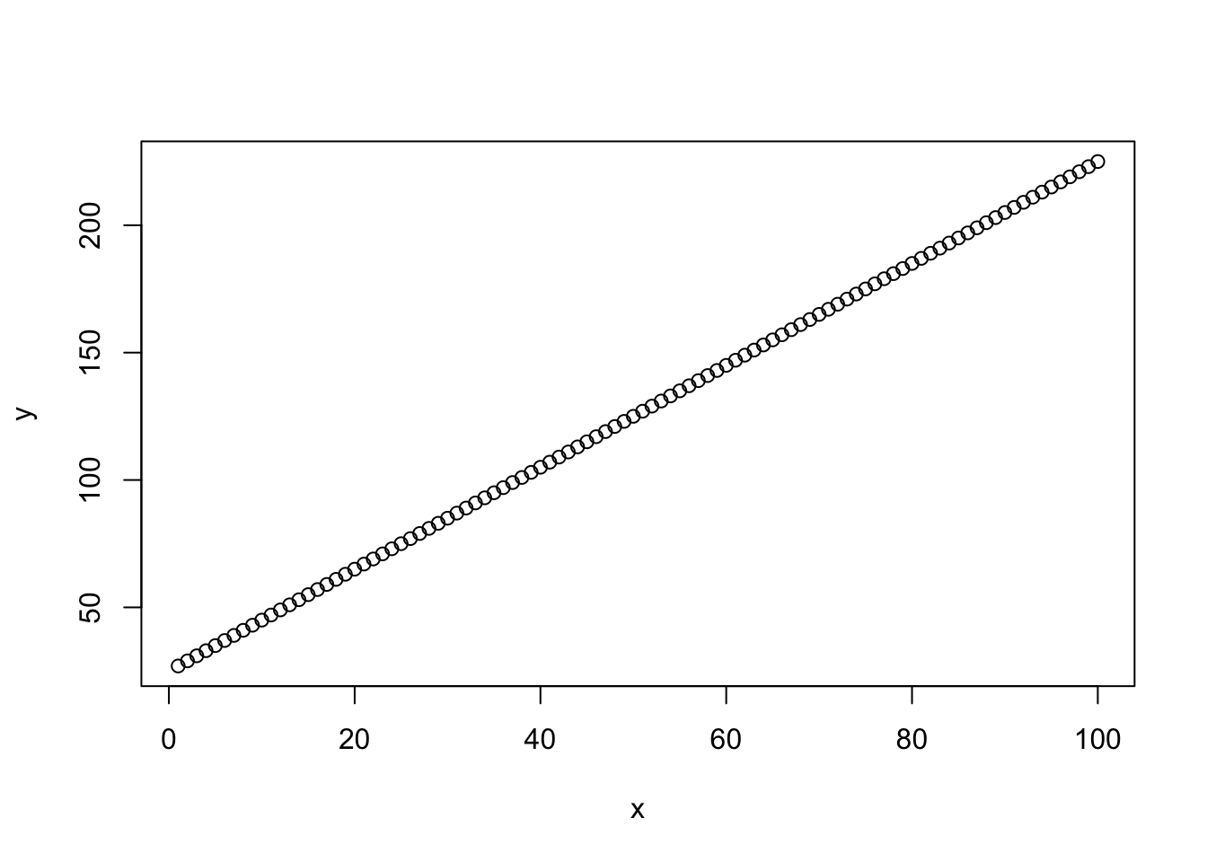
x.obs <- x + error.x
y.obs <- y + error.y
df <- data.frame(x = x.obs, y = y.obs)
ggplot(df, aes(x, y)) +
    geom_point()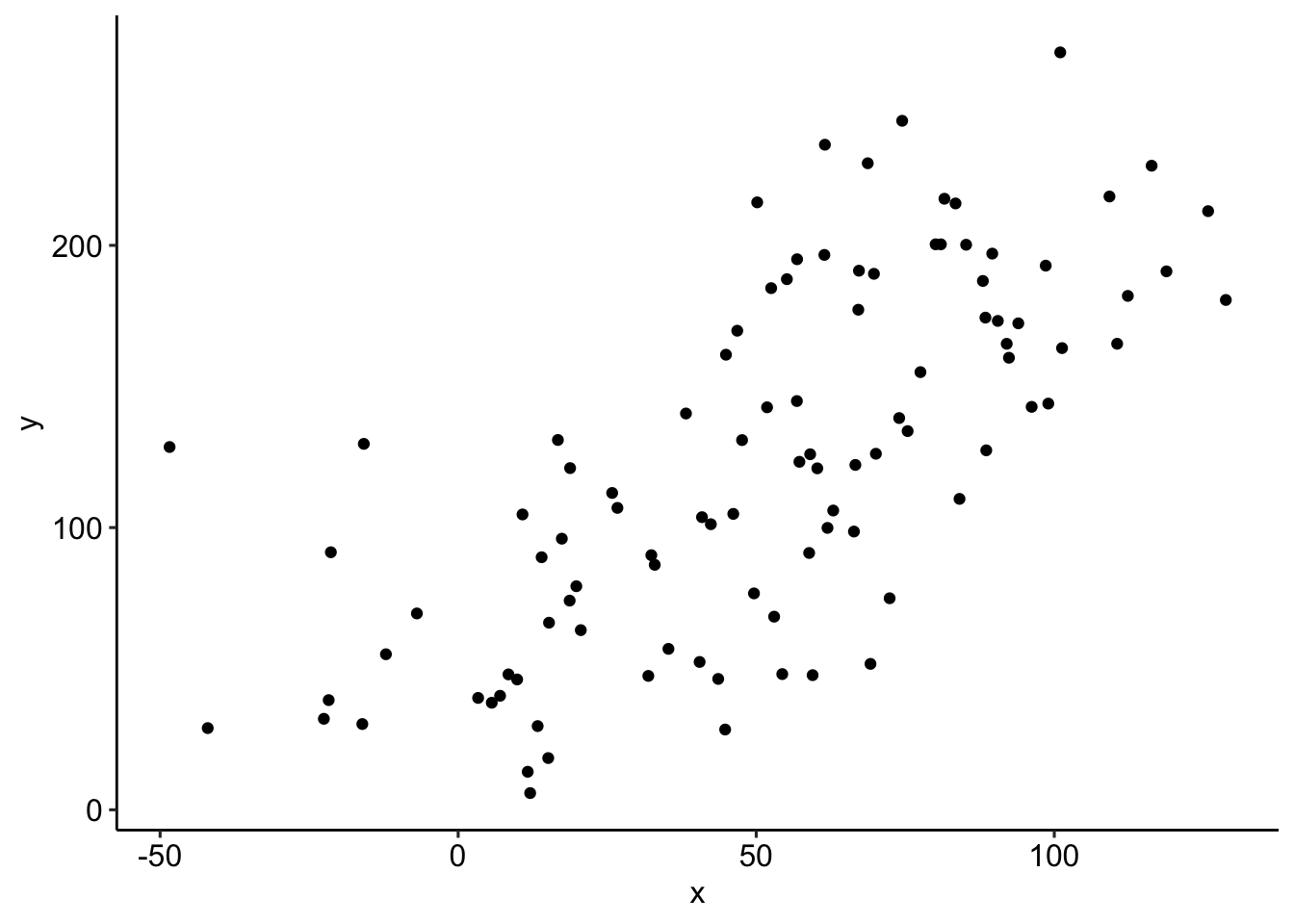
X.noncentered <- as.matrix(df)
X <- scale(X.noncentered, center=TRUE, scale=FALSE)
covX.calc <- t(X) %*% X/(nrow(X)-1)

# PCA
covX <- cov(X)
eig <- eigen(covX)
eigenVectors <- eig$vectors
eigenValues <- eig$values

singular.values <- svd(X)$d # sqrt(eigenValues * (nrow(X)-1)) --> WHY?
singular.vectors <- svd(X)$v


frames <- lapply(1:179, function(alpha) {
    w <- c(cos(alpha * pi/180), sin(alpha * pi/180))
    z <- X %*% (w %*% t(w))

    projected_values <- X %*% w
    variance_projected <- var(projected_values)

    data.frame(
        x = X[,1], y = X[,2],
        zx = z[,1], zy = z[,2],
        alpha = alpha,
        variance = variance_projected
    )
})

anim_data <- do.call(rbind, frames)

eig_df <- data.frame(x = c(0, 0),
                     y = c(0, 0),
                     xend = eigenVectors[1,] * sqrt(eigenValues),
                     yend = eigenVectors[2,] * sqrt(eigenValues),
                     col = c("PC1", "PC2"))


linear_fit <- lm(y~x, data = as.data.frame(X))
linear_fit.pred <- predict(linear_fit, newdata = as.data.frame(X)[,1,drop=FALSE])
linear_fit.pred.df <- data.frame(X=X[,1],Y=linear_fit.pred)
linear_fit.pred.df$col <- "linear fit"
Plot PCs
ggplot() +
    geom_point(aes(X[,1], X[,2]), color="blue", alpha=0.5) +
    geom_segment(data=eig_df,
                 aes(x=x, y=y, xend=xend, yend=yend, col=col),
                 arrow=arrow(length=unit(0.3,"cm")), size=1) +
    scale_color_manual(values=c("PC1"="red", "PC2"="green",`linear fit`="black"))+
    theme_minimal() +
    coord_equal() +
    xlab("X") +
    ylab("Y")
Warning: Using `size` aesthetic for lines was deprecated in ggplot2 3.4.0.
ℹ Please use `linewidth` instead.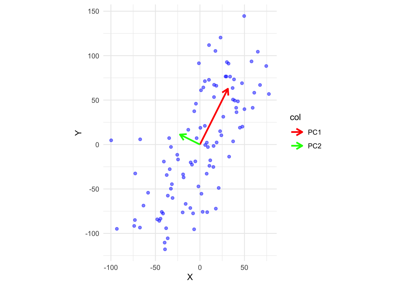
How does it compare with linear fit?
ggplot() +
    geom_point(aes(X[,1], X[,2]), color="blue", alpha=0.5) +
    geom_segment(data=eig_df,
                 aes(x=x, y=y, xend=xend, yend=yend, color=col),
                 arrow=arrow(length=unit(0.3,"cm")), size=1) +
        scale_color_manual(values=c("PC1"="red", "PC2"="green",`linear fit`="black"))+

    geom_line(data = linear_fit.pred.df, aes(X,Y, color=col))+
    theme_minimal() +
    coord_equal() +
    xlab("X") +
    ylab("Y")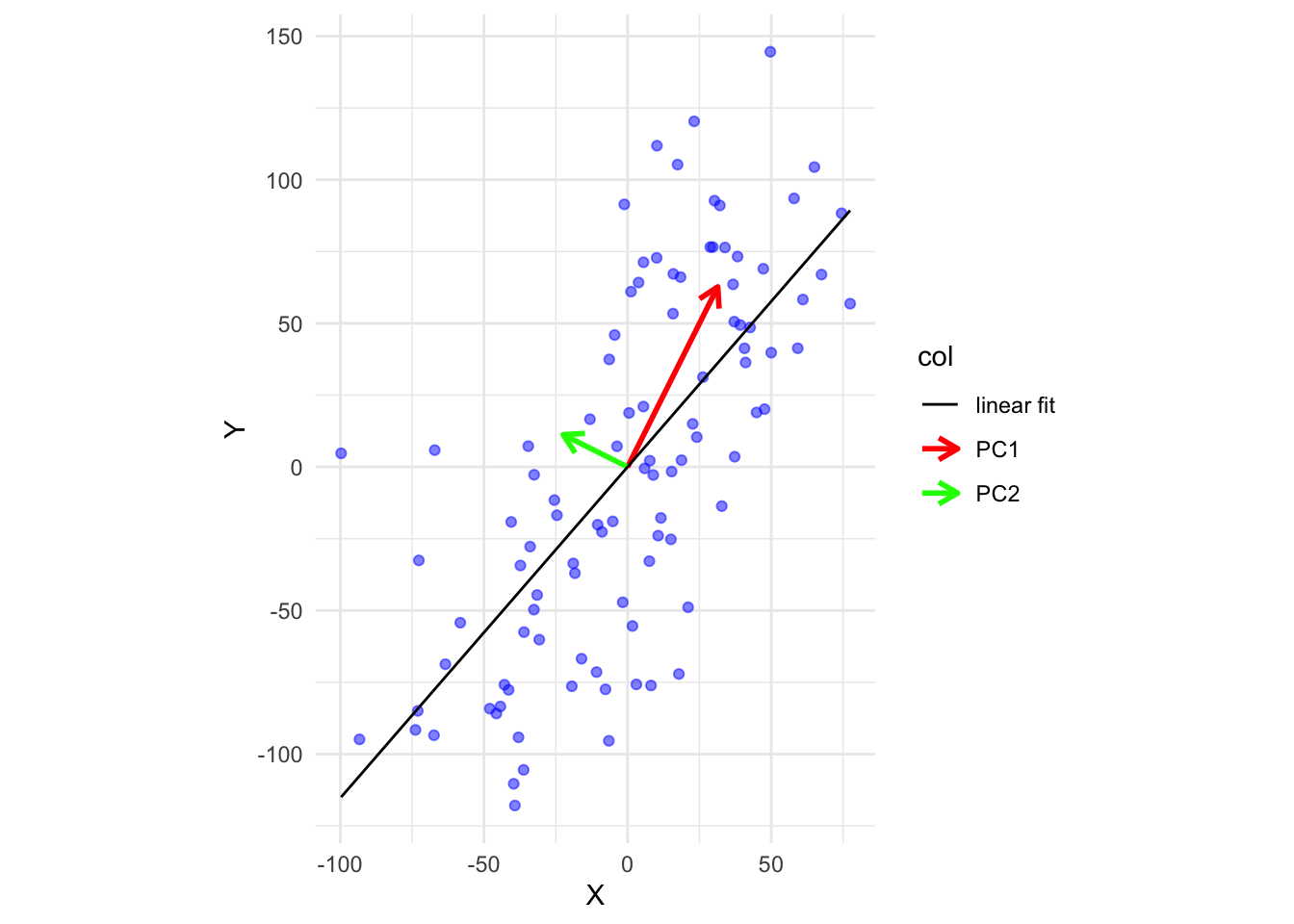
Animate
p <- ggplot(anim_data, aes(x, y)) +
    geom_point(color='blue', alpha=1) +
    geom_point(aes(zx, zy), color='red', size=2, alpha=1) +
    geom_segment(data=eig_df,
                 aes(x=x, y=y, xend=xend, yend=yend, color=col),
                 arrow=arrow(length=unit(0.3,"cm")), size=1) +
    scale_color_manual(values=c("PC1"="red", "PC2"="green"))+

    geom_segment(aes(xend=zx, yend=zy), color='red', alpha=0.5) +
    geom_abline(aes(intercept=0, slope=tan(alpha * pi/180)), color='gray', linetype="dashed") +

    geom_text(aes(x = Inf, y = Inf, label = paste("Variance:", round(variance, 2))),
              hjust = 1.1, vjust = 1.1, size = 4, color = "black",
              fontface = "bold") +

    geom_rect(aes(xmin = max(x) * 0.7, xmax = max(x) * 0.7 + variance/max(variance) * max(x) * 0.25,
                  ymin = max(y) * 0.85, ymax = max(y) * 0.9),
              fill = "orange", alpha = 0.7) +

    coord_equal() +
    transition_states(alpha, transition_length=2, state_length=2)
animate(p, fps=10, duration=10,
        width=8, height=5, units = "in", res = 150*2,
        renderer=gifski_renderer("pca_rotation.gif"))
Credits
Making sense of PCA by amoeba: https://stats.stackexchange.com/a/140579
What is principal component analysis? - Lior Pachter https://liorpachter.wordpress.com/2014/05/26/what-is-principal-component-analysis/