# run in terminal
# tar -xvf GSE135251_RAW.tarLecture 13: Analysis of bulk RNA-seq data: Signatures of Fibrosis
How should I run this notebook?
The easiest way to run each of the steps in this notebook is to download the raw file here, open it in Rstudio and run each code block one by one. Note that you need to also have Quarto installed to run this. Alternatively, you can also copy paste code blocks from this notebook either in your R console, R script or in an Rmarkdown file.
Fatty liver disease
We will be working on a dataset generated by Govaere et al. 2023 which is available on GEO.
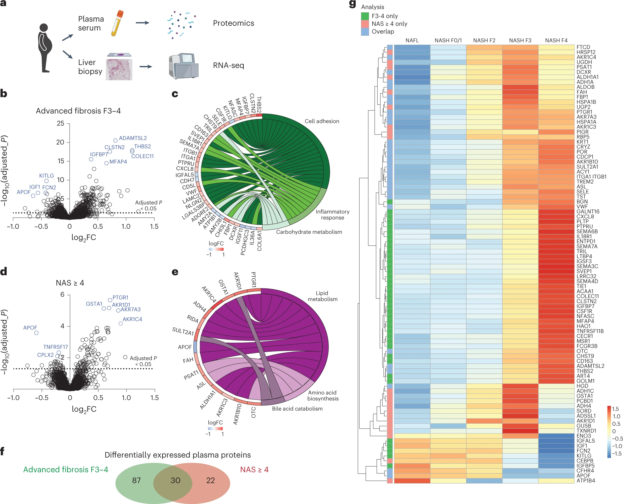
The paper uses RNA-seq data and proteomics to identify a gene signature associated with Non-alcoholic fatty liver disease (NAFLD) and its progression to cirrhosis. We will do an exploratory analysis of the data and identify gene signatures associated with different stages (severity) of the disease.
Here is the abstract:
Non-alcoholic fatty liver disease (NAFLD) is a common, progressive liver disease strongly associated with the metabolic syndrome. It is unclear how progression of NAFLD towards cirrhosis translates into systematic changes in circulating proteins. Here, we provide a detailed proteo-transcriptomic map of steatohepatitis and fibrosis during progressive NAFLD. In this multicentre proteomic study, we characterize 4,730 circulating proteins in 306 patients with histologically characterized NAFLD and integrate this with transcriptomic analysis in paired liver tissue. We identify circulating proteomic signatures for active steatohepatitis and advanced fibrosis, and correlate these with hepatic transcriptomics to develop a proteo-transcriptomic signature of 31 markers. Deconvolution of this signature by single-cell RNA sequencing reveals the hepatic cell types likely to contribute to proteomic changes with disease progression. As an exemplar of use as a non-invasive diagnostic, logistic regression establishes a composite model comprising four proteins (ADAMTSL2, AKR1B10, CFHR4 and TREM2), body mass index and type 2 diabetes mellitus status, to identify at-risk steatohepatitis.
Download the data
You can either go to the GEO page and download the data under the “Supplementary File section” or use the following code to download the data directly from your terminal.
The above command will download a file ‘GSE135251_RAW.tar’ in your directory. You can extract the files using the following command:
The data deposited on GEO is the the raw counts of the RNA-seq. Before we take a look at the counts, we will go through the process of aligning the raw reads to the transcriptome and generating the counts for one of the samples. You already have the ‘GenomicsWorkshop_fastqs.zip’ file downloaded on your machines. Let’s extract the files and take a look at the fastq files. All the commands in the section below are to be run in your terminal before we switch to R.
# run in terminal
wget -c "http://10.198.63.17:8000/GenomicsWorkshop_fastqs.zip"
unzip GenomicsWorkshop_fastqs.zip
cd GenomicsWorkshop_fastqs
Let’s look into what is inside the zip directory:
# run in terminal
ls -lh
-rw-rw-r– 1 saket saket 1.4G Dec 10 2020 SRR9883171_1.fastq.gz -rw-rw-r– 1 saket saket 1.4G Dec 10 2020 SRR9883171_2.fastq.gz
We will use the SRR9883171_1.fastq.gz and SRR9883171_2.fastq.gz files to align the reads to the transcriptome. We will use the cdna file you already downloaded to map the raw reads to the transcriptome.
# run in terminal
wget -c "https://ftp.ensembl.org/pub/release-115/fasta/homo_sapiens/cdna/Homo_sapiens.GRCh38.cdna.all.fa.gz"
Basics of bash scripting
Before we do that, we should look at some basic things that you would want to do with your fastq files.
1. What is the size of your fastq files?
# run in terminal
ls -ltrha
-rw-rw-r– 1 saket saket 1.4G Dec 10 2020 SRR9883171_2.fastq.gz -rw-rw-r– 1 saket saket 1.4G Dec 10 2020 SRR9883171_1.fastq.gz
2.How many reads does your data have?
# run in terminal
mamba install bc
echo $(zcat SRR9883171_1.fastq.gz|wc -l)/4|bc
33728028
# run in terminal
echo $(zcat SRR9883171_2.fastq.gz|wc -l)/4|bc
33728028
3. What is the length of reads? Are R1 and R2 read lengths same?
# run in terminal
zcat SRR9883171_1.fastq.gz | head -n 5
@SRR9883171.1 1/1 GGAAGCTGCCCGGCGGGTCATGGGAATAACGCCGCCGCATCGCCGGTCGGCATCGTTTATGGTCGGAACTACGACG + AAAAAEEEEEEEEEEEEEEEEEEEEEEEEEEEEEEEEEEEEEEEEEEEEEEAEEEEEEEEEEEEEEEEEEAEE/EE @SRR9883171.2 2/1
# run in terminal
zcat SRR9883171_2.fastq.gz | head -n 5
@SRR9883171.1 1/2 ACGGNNNNNNNNNNNNNNNNNNNNNNNNNNNNNNNNNNNNNNNNNNNNNNNNNNNNNNNNNNNNNNNNNNNNNNNN + AAAA######################################################################## @SRR9883171.2 2/2
# run in terminal
zcat SRR9883171_1.fastq.gz  | head -n 2  | tail -n 1 | tr -d '\n' | wc -c
76
# run in terminal
!zcat SRR9883171_2.fastq.gz  | head -n 2  | tail -n 1 | tr -d '\n' | wc -c
76
4. How many reads have Ns (one or more) in them?
# run in terminal
zcat SRR9883171_1.fastq.gz | awk 'NR%4==2' | grep -c 'N'
4561
Quality control checks
Before we do any pre-processing it is always a good idea to take a quick look the quality score description. We will run FastQC to run quality checks for our sequencing data
# run in terminal
mamba install fastqc
fastqc SRR9883171_1.fastq.gz SRR9883171_2.fastq.gz
Generating kallisto index
Once our basic quality control checks are done, we can start mapping using kallisto. We will first generate the index for the transcriptome.
# run in terminal
mamba install kallisto
kallisto index -t 8 -i human_cdna.idx Homo_sapiens.GRCh38.cdna.all.fa.gz
Next, we use this index to map the raw sequences:
# run in terminal
kallisto quant -i human_cdna.idx -o output/ -t 12 GenomicsWorkshop_fastqs/SRR9883171_1.fastq.gz GenomicsWorkshop_fastqs/SRR9883171_2.fastq.gz
Once finished, you can check the files it generates
# run in terminal
cd output
ls -ltrha
-rw-rw-r– 1 saket 450 Mar 1 04:55 run_info.json drwxrwxr-x 5 saket 160 Mar 1 04:55 . -rw-rw-r– 1 saket 8.0M Mar 1 04:55 abundance.tsv -rw-rw-r– 1 saket 2.6M Mar 1 04:55 abundance.h5
Let’s look into abundance.tsv:
# run in terminal
head abundance.tsv
target_id length eff_length est_counts tpm ENST00000390473.1 51 9.5 1 4.04028 ENST00000390484.1 60 11.4333 0 0 ENST00000390488.1 56 10.2174 0 0 ENST00000390476.1 59 11.5926 0 0 ENST00000390489.1 63 11.8667 0 0
So the quantifications are at the transcript level, we would ideally want them at the gene level. To do this, we need mapping from the transcripts (isoforms) to the gene ids (and gene names). Let’s go back to the cdna file and see its contents:
# run in terminal
 zcat scripts/Homo_sapiens.GRCh38.cdna.all.fa.gz| head
ENST00000390473.1 cdna chromosome:GRCh38:14:22450089:22450139:1 gene:ENSG00000211825.1 gene_biotype:TR_J_gene transcript_biotype:TR_J_gene gene_symbol:TRDJ1 description:T cell receptor delta joining 1 [Source:HGNC Symbol;Acc:HGNC:12257] ACACCGATAAACTCATCTTTGGAAAAGGAACCCGTGTGACTGTGGAACCAA ENST00000390484.1 cdna chromosome:GRCh38:14:22482287:22482346:1 gene:ENSG00000211836.1 gene_biotype:TR_J_gene transcript_biotype:TR_J_gene gene_symbol:TRAJ54 description:T cell receptor alpha joining 54 [Source:HGNC Symbol;Acc:HGNC:12086] TAATTCAGGGAGCCCAGAAGCTGGTATTTGGCCAAGGAACCAGGCTGACTATCAACCCAA
So, we can extract the transcript id, gene id and gene name using the 1st, 4th and 7th column. We also need to track which position within these columns does our id start.
# run in terminal
zcat Homo_sapiens.GRCh38.cdna.all.fa.gz| \
grep '>' |
awk '{FS= " "}BEGIN{ print "tx_id,gene_id,gene_name"};{print substr($1,2) "," substr($4,6) "," substr($7,13)};' >
 t2g.csv
Since we mapped the raw data, we would also like to ideally know what are some metadata files associated with the sample run SRR9883171, we can use pysradb to download the entire metadata of this project:
# run in terminal
pysradb metadata SRP217231 --detailed --saveto SRP217231_metadata.tsv
We can now look at what is the metadata corresponding to the run ‘SRR9883171’ which we mapped:
# run in terminal
cat SRP217231_metadata.tsv| grep SRR9883171
SRR9883171 SRP217231 TRANSCRIPTOMIC PROFILING ACROSS THE SPECTRUM OF NON-ALCOHOLIC FATTY LIVER DISEASESRX6635692 GSM3998382: Liver patient 138; Homo sapiens; RNA-Seq GSM3998382: Liver patient 138; Homo sapiens; RNA-Seq 9606 Homo sapiens RNA-Seq TRANSCRIPTOMIC cDNA PAIRED SRS5207152 SAMN12426209 PRJNA558102 NextSeq 500 NextSeq 500 ILLUMINA 33728028 2045452993 33728028 5092636819 GSM3998382_r1 SRR9883171.lite https://sra-downloadb.be-md.ncbi.nlm.nih.gov/sos3/sra-pub-zq-22/SRR009/9883/SRR9883171/SRR9883171.lite.1 1339338918 2022-07-16 00:36:31 f75d33d154344352ab7bfa32f81f8f42 1 SRA Lite Primary ETL 1 s3://sra-pub-zq-4/SRR9883171/SRR9883171.lite.1 s3.us-east-1 aws identity https://sra-downloadb.be-md.ncbi.nlm.nih.gov/sos3/sra-pub-zq-22/SRR009/9883/SRR9883171/SRR9883171.lite.1 worldwide anonymous gs://sra-pub-zq-103/SRR9883171/SRR9883171.lite.1 gs.us-east1 gcp identity GSM3998382 NAFLD_moderate_liver biopsy 7 3 NASH_F3 NAFLD moderatehttp://ftp.sra.ebi.ac.uk/vol1/fastq/SRR988/001/SRR9883171/SRR9883171_1.fastq.gz http://ftp.sra.ebi.ac.uk/vol1/fastq/SRR988/001/SRR9883171/SRR9883171_2.fastq.gz era-fasp@fasp.sra.ebi.ac.uk:vol1/fastq/SRR988/001/SRR9883171/SRR9883171_1.fastq.gz era-fasp@fasp.sra.ebi.ac.uk:vol1/fastq/SRR988/001/SRR9883171/SRR9883171_2.fastq.gz
Among other things, GSM3998382 corresponds to SRR9883171 and came from a NAFLD_moderate_liver biopsy sample.
Analysis of kallisto counts
library(tidyverse)── Attaching core tidyverse packages ──────────────────────── tidyverse 2.0.0 ──
✔ dplyr 1.1.4 ✔ readr 2.1.5
✔ forcats 1.0.1 ✔ stringr 1.5.2
✔ ggplot2 4.0.0 ✔ tibble 3.3.0
✔ lubridate 1.9.4 ✔ tidyr 1.3.1
✔ purrr 1.1.0
── Conflicts ────────────────────────────────────────── tidyverse_conflicts() ──
✖ dplyr::filter() masks stats::filter()
✖ dplyr::lag() masks stats::lag()
ℹ Use the conflicted package (<http://conflicted.r-lib.org/>) to force all conflicts to become errorslibrary(ggpubr)
theme_set(theme_pubr())
# change file paths as required
geo.counts <- read_tsv("data/bulk/GSM3998232_17_82.counts.txt.gz", col_names = c("gene_id", "geo_counts")) Rows: 64258 Columns: 2
── Column specification ────────────────────────────────────────────────────────
Delimiter: "\t"
chr (1): gene_id
dbl (1): geo_counts
ℹ Use `spec()` to retrieve the full column specification for this data.
ℹ Specify the column types or set `show_col_types = FALSE` to quiet this message.head(geo.counts)# A tibble: 6 × 2
gene_id geo_counts
<chr> <dbl>
1 ENSG00000000003 1278
2 ENSG00000000005 4
3 ENSG00000000419 217
4 ENSG00000000457 300
5 ENSG00000000460 61
6 ENSG00000000938 144Read the t2g file (we need this to collapse the transcript counts to gene counts):
# change file paths as required

t2g <- read_csv("DH607_RNAHandson/t2g.csv")
Warning: One or more parsing issues, call `problems()` on your data frame for details,
e.g.:
dat <- vroom(...)
problems(dat)Rows: 207133 Columns: 3
── Column specification ────────────────────────────────────────────────────────
Delimiter: ","
chr (3): tx_id, gene_id, gene_name
ℹ Use `spec()` to retrieve the full column specification for this data.
ℹ Specify the column types or set `show_col_types = FALSE` to quiet this message.head(t2g)# A tibble: 6 × 3
tx_id gene_id gene_name
<chr> <chr> <chr>
1 ENST00000390473.1 ENSG00000211825.1 TRDJ1
2 ENST00000390484.1 ENSG00000211836.1 TRAJ54
3 ENST00000390488.1 ENSG00000211840.1 TRAJ49
4 ENST00000390476.1 ENSG00000211828.1 TRDJ3
5 ENST00000390489.1 ENSG00000211841.1 TRAJ48
6 ENST00000390480.2 ENSG00000211832.2 TRAJ59 Read the counts that we generated using kallisto
# change file paths as required
kallisto.tx.counts <- read_tsv("DH607_RNAHandson/output/abundance.tsv")
Rows: 207133 Columns: 5
── Column specification ────────────────────────────────────────────────────────
Delimiter: "\t"
chr (1): target_id
dbl (4): length, eff_length, est_counts, tpm
ℹ Use `spec()` to retrieve the full column specification for this data.
ℹ Specify the column types or set `show_col_types = FALSE` to quiet this message.head(kallisto.tx.counts)# A tibble: 6 × 5
target_id length eff_length est_counts tpm
<chr> <dbl> <dbl> <dbl> <dbl>
1 ENST00000390473.1 51 9.5 1 4.04
2 ENST00000390484.1 60 11.4 0 0
3 ENST00000390488.1 56 10.2 0 0
4 ENST00000390476.1 59 11.6 0 0
5 ENST00000390489.1 63 11.9 0 0
6 ENST00000390480.2 54 10.4 0 0 # change file paths as required
kallisto.gene.counts <- kallisto.tx.counts %>%
inner_join(t2g, by = c("target_id" = "tx_id")) %>%
mutate(gene_id = str_replace(gene_id, "\\..*", "")) %>% # remove .1, .2 etc
group_by(gene_id, gene_name) %>% # group by gene id
summarise(kallisto_counts = sum(est_counts)) %>% # sum the counts across all isoforms of a gene
ungroup() `summarise()` has grouped output by 'gene_id'. You can override using the
`.groups` argument.kallisto.geo.counts <- full_join(kallisto.gene.counts, geo.counts)Joining with `by = join_by(gene_id)`library(ggpubr)
ggplot(kallisto.geo.counts, aes(x = kallisto_counts, y = geo_counts)) +
geom_point() +
geom_abline() +
labs(x = "Kallisto counts", y = "GEO counts") +
scale_x_log10() +
scale_y_log10() +
theme_pubr()Warning in scale_x_log10(): log-10 transformation introduced infinite values.Warning in scale_y_log10(): log-10 transformation introduced infinite values.Warning: Removed 30082 rows containing missing values or values outside the scale range
(`geom_point()`).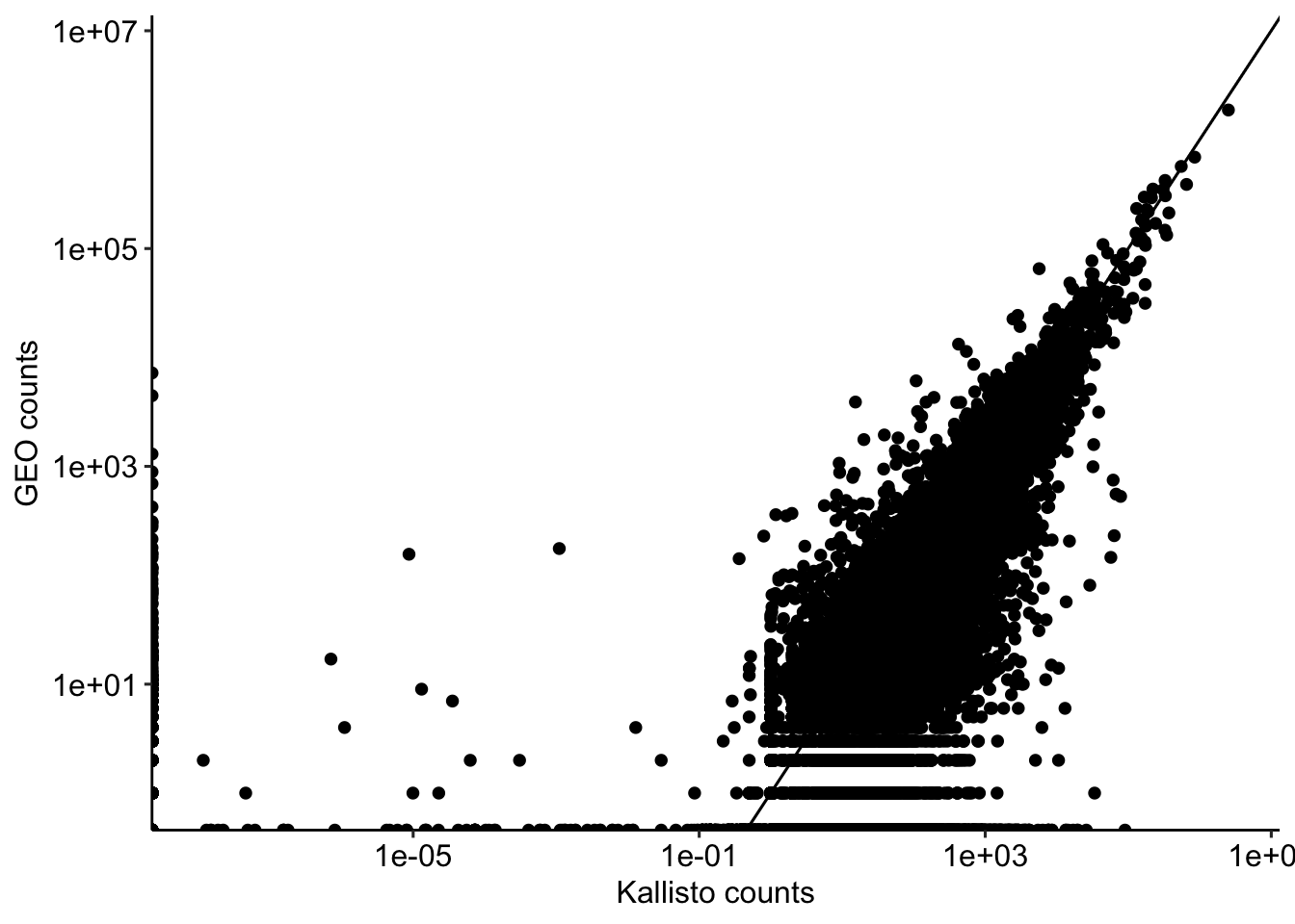
kallisto.geo.counts.inner <- inner_join(kallisto.gene.counts, geo.counts)Joining with `by = join_by(gene_id)`cor(kallisto.geo.counts.inner$kallisto_counts, kallisto.geo.counts.inner$geo_counts)[1] 0.9704097So we are getting a correlation of 0.97 between the kallisto counts and the counts from GEO. This is a good sign that our quantification is close to what authors did, but there are differences also. We will ignore the differences here for simplicity and for the rest of the analysis focus on working off the files that was generated by the authors.
All the counts from all the samples have been summarized in this file that you can download and use for the rest of the analysis.
Differential expression analysis
#z <- lapply(X = list.files("data/bulk/", pattern = "*.gz"))
#df.list <- list()
#for (f in list.files("data/bulk/", pattern = "*.gz")){
#    df <- read_csv(file = paste0("Data/bulk/",f)s )
#    df.list[[]]
#}

counts <- read_csv("data/bulk/all_counts.csv") %>% as.data.frame()
Rows: 62657 Columns: 217
── Column specification ────────────────────────────────────────────────────────
Delimiter: ","
chr (1): gene_name
dbl (216): GSM3998167, GSM3998168, GSM3998169, GSM3998170, GSM3998171, GSM39...
ℹ Use `spec()` to retrieve the full column specification for this data.
ℹ Specify the column types or set `show_col_types = FALSE` to quiet this message.head(counts) gene_name GSM3998167 GSM3998168 GSM3998169 GSM3998170 GSM3998171 GSM3998172
1 TSPAN6 2565 2400 2391 2835 3099 2214
2 TNMD 0 14 0 0 0 7
3 DPM1 605 525 709 671 869 500
4 SCYL3 315 330 329 418 348 347
5 C1orf112 92 89 115 97 108 65
6 FGR 96 91 292 115 144 154
GSM3998173 GSM3998174 GSM3998175 GSM3998176 GSM3998177 GSM3998178 GSM3998179
1 2904 1823 1627 2285 2513 1892 2315
2 1 3 3 7 35 0 3
3 675 440 316 472 581 497 514
4 337 209 276 367 407 336 294
5 102 91 48 81 242 69 67
6 132 160 49 76 83 82 139
GSM3998180 GSM3998181 GSM3998182 GSM3998183 GSM3998184 GSM3998185 GSM3998186
1 2484 2038 1926 2947 2613 3010 2127
2 0 0 14 0 4 12 2
3 593 433 329 697 655 690 579
4 358 315 383 293 433 341 441
5 127 55 65 117 83 109 123
6 84 91 70 152 113 96 85
GSM3998187 GSM3998188 GSM3998189 GSM3998190 GSM3998191 GSM3998192 GSM3998193
1 2767 3072 2326 2525 2276 1987 2148
2 2 30 2 0 0 0 2
3 643 665 546 425 630 473 635
4 376 337 340 350 439 320 336
5 124 161 80 71 150 56 99
6 185 164 83 116 118 124 147
GSM3998194 GSM3998195 GSM3998196 GSM3998197 GSM3998198 GSM3998199 GSM3998200
1 1938 3029 1755 3110 3402 2914 2713
2 0 0 0 0 8 0 0
3 558 716 499 972 793 655 631
4 345 317 282 374 422 417 358
5 163 47 43 135 136 102 101
6 208 100 100 96 194 179 76
GSM3998201 GSM3998202 GSM3998203 GSM3998204 GSM3998205 GSM3998206 GSM3998207
1 2105 2192 2208 2162 1877 2163 2399
2 1 1 1 0 0 0 0
3 462 566 551 354 468 878 730
4 338 331 335 269 291 299 415
5 43 65 143 74 103 65 124
6 96 111 74 106 102 87 98
GSM3998208 GSM3998209 GSM3998210 GSM3998211 GSM3998212 GSM3998213 GSM3998214
1 2620 1978 1718 2195 2595 3128 2398
2 0 4 1 0 0 0 0
3 611 779 410 539 634 675 452
4 270 325 270 326 318 504 341
5 36 119 59 58 103 129 125
6 60 86 103 95 127 156 170
GSM3998215 GSM3998216 GSM3998217 GSM3998218 GSM3998219 GSM3998220 GSM3998221
1 2653 2531 2317 1881 2519 2588 1928
2 1 5 0 5 8 6 2
3 854 529 374 376 521 379 453
4 357 401 309 377 337 276 460
5 87 51 94 169 57 127 158
6 93 171 87 128 139 123 127
GSM3998222 GSM3998223 GSM3998224 GSM3998225 GSM3998226 GSM3998227 GSM3998228
1 1690 2400 1847 3143 2660 1084 2889
2 0 16 1 4 0 1 4
3 439 430 352 661 581 346 584
4 255 278 179 418 417 308 404
5 141 89 56 132 111 68 82
6 76 170 109 320 192 110 194
GSM3998229 GSM3998230 GSM3998231 GSM3998232 GSM3998233 GSM3998234 GSM3998235
1 1765 1243 1937 1278 1566 1722 2755
2 0 0 4 4 0 0 2
3 479 275 476 217 425 399 577
4 277 259 353 300 335 296 351
5 61 86 78 61 102 91 100
6 166 58 99 144 174 178 122
GSM3998236 GSM3998237 GSM3998238 GSM3998239 GSM3998240 GSM3998241 GSM3998242
1 1970 1983 1204 2371 1379 2080 1428
2 3 0 9 1 1 3 0
3 435 583 279 537 421 555 218
4 376 267 288 334 311 369 242
5 90 77 105 138 76 76 50
6 128 77 180 87 127 121 80
GSM3998243 GSM3998244 GSM3998245 GSM3998246 GSM3998247 GSM3998248 GSM3998249
1 1558 1610 2095 1613 3828 2609 2456
2 1 1 0 0 1 0 2
3 319 417 492 457 723 599 766
4 290 341 328 364 381 461 483
5 65 35 158 126 103 95 117
6 130 183 178 218 105 148 108
GSM3998250 GSM3998251 GSM3998252 GSM3998253 GSM3998254 GSM3998255 GSM3998256
1 3065 3499 2194 1777 2745 2660 2197
2 11 3 0 0 6 0 2
3 654 650 433 326 481 486 496
4 427 380 378 308 418 415 265
5 108 95 61 78 72 88 92
6 151 161 173 103 117 150 136
GSM3998257 GSM3998258 GSM3998259 GSM3998260 GSM3998261 GSM3998262 GSM3998263
1 2074 2735 796 1225 3672 2737 3350
2 0 2 0 0 2 1 5
3 543 593 192 248 655 547 714
4 432 449 156 380 346 400 355
5 136 206 68 70 91 73 77
6 217 133 44 113 108 105 182
GSM3998264 GSM3998265 GSM3998266 GSM3998267 GSM3998268 GSM3998269 GSM3998270
1 3311 2699 2277 3511 1412 2882 3302
2 1 0 4 1 0 7 3
3 556 511 382 626 247 578 631
4 419 333 327 366 232 402 437
5 100 118 50 78 61 101 108
6 120 112 88 75 83 148 161
GSM3998271 GSM3998272 GSM3998273 GSM3998274 GSM3998275 GSM3998276 GSM3998277
1 3437 1415 1253 2289 2870 2121 1522
2 0 2 9 0 10 66 0
3 703 331 239 556 400 563 211
4 422 311 198 282 329 198 219
5 185 47 61 97 89 49 57
6 145 227 74 113 69 110 88
GSM3998278 GSM3998279 GSM3998280 GSM3998281 GSM3998282 GSM3998283 GSM3998284
1 1261 2084 558 2407 2356 1325 1644
2 0 1 0 0 1 0 1
3 255 443 65 520 649 262 329
4 189 338 108 374 385 353 210
5 66 117 40 123 51 123 99
6 92 154 152 95 127 100 78
GSM3998285 GSM3998286 GSM3998287 GSM3998288 GSM3998289 GSM3998290 GSM3998291
1 1095 2908 2764 2314 3077 3265 2976
2 0 27 33 0 3 0 1
3 248 576 568 400 524 813 595
4 194 402 397 353 383 493 385
5 73 87 141 123 97 238 96
6 159 131 95 49 84 228 163
GSM3998292 GSM3998293 GSM3998294 GSM3998295 GSM3998296 GSM3998297 GSM3998298
1 2149 1503 2618 2904 3579 2906 3466
2 0 19 2 1 6 17 0
3 358 335 408 474 634 596 544
4 330 270 310 337 401 319 361
5 79 60 56 84 108 52 51
6 119 114 53 116 84 67 128
GSM3998299 GSM3998300 GSM3998301 GSM3998302 GSM3998303 GSM3998304 GSM3998305
1 2880 3145 3693 2374 1948 2640 3161
2 2 1 1 0 0 0 1
3 562 648 649 440 405 668 549
4 338 387 474 301 242 281 483
5 94 111 160 59 60 42 118
6 64 113 197 64 72 72 108
GSM3998306 GSM3998307 GSM3998308 GSM3998309 GSM3998310 GSM3998311 GSM3998312
1 2353 1915 2765 3070 1952 3660 2750
2 2 14 1 4 8 6 0
3 469 580 670 814 465 720 678
4 260 453 387 376 310 402 381
5 63 151 97 132 131 202 59
6 87 111 129 88 81 98 106
GSM3998313 GSM3998314 GSM3998315 GSM3998316 GSM3998317 GSM3998318 GSM3998319
1 2868 3784 3935 3507 3832 4527 1896
2 0 1 3 0 0 0 1
3 559 797 806 812 876 948 364
4 329 405 404 394 378 431 325
5 91 88 78 119 136 94 33
6 138 91 75 74 109 127 81
GSM3998320 GSM3998321 GSM3998322 GSM3998323 GSM3998324 GSM3998325 GSM3998326
1 3225 2403 3181 2828 2818 3552 2575
2 2 3 2 4 15 0 2
3 769 447 630 837 954 658 561
4 364 367 349 411 453 399 320
5 120 157 64 69 93 151 117
6 87 118 99 97 152 93 66
GSM3998327 GSM3998328 GSM3998329 GSM3998330 GSM3998331 GSM3998332 GSM3998333
1 3078 3520 2108 1885 1889 2158 1658
2 0 0 11 0 0 0 0
3 787 807 625 432 487 464 407
4 406 430 471 310 278 363 286
5 113 117 173 108 234 74 66
6 148 105 513 67 102 227 56
GSM3998334 GSM3998335 GSM3998336 GSM3998337 GSM3998338 GSM3998339 GSM3998340
1 3108 2081 2539 3289 2196 2828 2624
2 30 0 0 1 3 0 0
3 744 434 466 691 439 472 511
4 444 305 296 398 276 507 518
5 217 82 46 77 80 89 158
6 187 150 77 120 55 121 90
GSM3998341 GSM3998342 GSM3998343 GSM3998344 GSM3998345 GSM3998346 GSM3998347
1 1765 2480 1124 1516 1025 1679 1193
2 4 0 0 3 2 2 0
3 222 388 239 353 236 312 305
4 117 278 214 272 191 230 204
5 35 99 27 40 38 39 84
6 47 57 151 107 144 176 89
GSM3998348 GSM3998349 GSM3998350 GSM3998351 GSM3998352 GSM3998353 GSM3998354
1 1525 1461 1484 1243 1542 1321 1293
2 0 0 0 4 1 3 0
3 337 213 308 234 394 299 327
4 289 242 252 250 269 191 260
5 68 88 46 62 53 20 55
6 148 176 168 221 141 102 123
GSM3998355 GSM3998356 GSM3998357 GSM3998358 GSM3998359 GSM3998360 GSM3998361
1 939 1221 1454 2129 1840 904 1072
2 0 3 0 1 1 2 0
3 287 275 361 344 396 286 214
4 178 255 229 347 348 199 143
5 59 45 48 56 97 51 54
6 191 158 146 196 167 162 115
GSM3998362 GSM3998363 GSM3998364 GSM3998365 GSM3998366 GSM3998367 GSM3998368
1 753 1403 1611 1315 1644 1435 1703
2 1 0 2 25 0 2 0
3 156 344 287 318 261 281 420
4 165 216 271 242 306 353 278
5 51 81 74 45 67 80 91
6 204 139 125 262 98 142 146
GSM3998369 GSM3998370 GSM3998371 GSM3998372 GSM3998373 GSM3998374 GSM3998375
1 931 2386 2414 2876 2251 1401 2168
2 0 6 0 16 0 0 0
3 177 546 628 663 474 364 507
4 175 359 340 391 324 260 354
5 31 67 88 78 67 126 76
6 122 224 182 179 193 177 138
GSM3998376 GSM3998377 GSM3998378 GSM3998379 GSM3998380 GSM3998381 GSM3998382
1 2096 2981 2269 2526 2010 1725 1660
2 0 1 1 4 11 12 0
3 525 713 366 607 572 336 353
4 335 410 250 417 310 291 320
5 81 89 120 122 84 67 49
6 209 206 213 206 153 215 244rownames(counts) <- make.unique(counts$gene_name)
counts$gene_name <- NULLWe will also need the metadata file that you generated using pysradb (also available here)
metadata <- read_tsv("data/bulk/SRP217231_metadata.tsv") %>% as.data.frame()Rows: 216 Columns: 56
── Column specification ────────────────────────────────────────────────────────
Delimiter: "\t"
chr (41): run_accession, study_accession, study_title, experiment_accession...
dbl (10): organism_taxid, total_spots, total_size, run_total_spots, run_tot...
lgl (4): library_name, sample_title, ena_fastq_http, ena_fastq_ftp
dttm (1): public_date
ℹ Use `spec()` to retrieve the full column specification for this data.
ℹ Specify the column types or set `show_col_types = FALSE` to quiet this message.head(metadata) run_accession study_accession
1 SRR9882956 SRP217231
2 SRR9882957 SRP217231
3 SRR9882958 SRP217231
4 SRR9882959 SRP217231
5 SRR9882960 SRP217231
6 SRR9882961 SRP217231
study_title
1 TRANSCRIPTOMIC PROFILING ACROSS THE SPECTRUM OF NON-ALCOHOLIC FATTY LIVER DISEASE
2 TRANSCRIPTOMIC PROFILING ACROSS THE SPECTRUM OF NON-ALCOHOLIC FATTY LIVER DISEASE
3 TRANSCRIPTOMIC PROFILING ACROSS THE SPECTRUM OF NON-ALCOHOLIC FATTY LIVER DISEASE
4 TRANSCRIPTOMIC PROFILING ACROSS THE SPECTRUM OF NON-ALCOHOLIC FATTY LIVER DISEASE
5 TRANSCRIPTOMIC PROFILING ACROSS THE SPECTRUM OF NON-ALCOHOLIC FATTY LIVER DISEASE
6 TRANSCRIPTOMIC PROFILING ACROSS THE SPECTRUM OF NON-ALCOHOLIC FATTY LIVER DISEASE
experiment_accession experiment_title
1 SRX6635477 GSM3998167: Liver patient 97; Homo sapiens; RNA-Seq
2 SRX6635478 GSM3998168: Liver patient 98; Homo sapiens; RNA-Seq
3 SRX6635479 GSM3998169: Liver patient 101; Homo sapiens; RNA-Seq
4 SRX6635480 GSM3998170: Liver patient 102; Homo sapiens; RNA-Seq
5 SRX6635481 GSM3998171: Liver patient 105; Homo sapiens; RNA-Seq
6 SRX6635482 GSM3998172: Liver patient 106; Homo sapiens; RNA-Seq
experiment_desc organism_taxid
1 GSM3998167: Liver patient 97; Homo sapiens; RNA-Seq 9606
2 GSM3998168: Liver patient 98; Homo sapiens; RNA-Seq 9606
3 GSM3998169: Liver patient 101; Homo sapiens; RNA-Seq 9606
4 GSM3998170: Liver patient 102; Homo sapiens; RNA-Seq 9606
5 GSM3998171: Liver patient 105; Homo sapiens; RNA-Seq 9606
6 GSM3998172: Liver patient 106; Homo sapiens; RNA-Seq 9606
organism_name library_name library_strategy library_source library_selection
1 Homo sapiens NA RNA-Seq TRANSCRIPTOMIC cDNA
2 Homo sapiens NA RNA-Seq TRANSCRIPTOMIC cDNA
3 Homo sapiens NA RNA-Seq TRANSCRIPTOMIC cDNA
4 Homo sapiens NA RNA-Seq TRANSCRIPTOMIC cDNA
5 Homo sapiens NA RNA-Seq TRANSCRIPTOMIC cDNA
6 Homo sapiens NA RNA-Seq TRANSCRIPTOMIC cDNA
library_layout sample_accession sample_title biosample bioproject
1 PAIRED SRS5206937 NA SAMN12426403 PRJNA558102
2 PAIRED SRS5206938 NA SAMN12426402 PRJNA558102
3 PAIRED SRS5206939 NA SAMN12426401 PRJNA558102
4 PAIRED SRS5206940 NA SAMN12426400 PRJNA558102
5 PAIRED SRS5206942 NA SAMN12426399 PRJNA558102
6 PAIRED SRS5206941 NA SAMN12426398 PRJNA558102
instrument instrument_model instrument_model_desc total_spots total_size
1 NextSeq 500 NextSeq 500 ILLUMINA 34975618 2056090366
2 NextSeq 500 NextSeq 500 ILLUMINA 30081230 1777224143
3 NextSeq 500 NextSeq 500 ILLUMINA 35765327 2098480575
4 NextSeq 500 NextSeq 500 ILLUMINA 41879270 2491421504
5 NextSeq 500 NextSeq 500 ILLUMINA 41594970 2520274624
6 NextSeq 500 NextSeq 500 ILLUMINA 36740685 2207445480
run_total_spots run_total_bases run_alias public_filename public_size
1 34975618 5277841961 GSM3998167_r1 SRR9882956.lite 1388241653
2 30081230 4539511521 GSM3998168_r1 SRR9882957.lite 1194716974
3 35765327 5398465979 GSM3998169_r1 SRR9882958.lite 1419931980
4 41879270 6319188516 GSM3998170_r1 SRR9882959.lite 1662792131
5 41594970 6276619633 GSM3998171_r1 SRR9882960.lite 1650884038
6 36740685 5544490945 GSM3998172_r1 SRR9882961.lite 1459212208
public_date public_md5 public_version
1 2022-08-05 02:01:24 3052734fbf1dc359aa6dc2173802941a 1
2 2022-07-05 22:47:28 d6f0c9c237484e9ccb59544b0fa4fbbd 1
3 2022-07-27 17:28:45 34bbc9116a0fc1c414d01b51c451c407 1
4 2022-07-16 00:36:40 d66a5846b68ac646a9930be78ad9d9fe 1
5 2022-07-09 19:01:18 79a5568e513a2335174acd310d600dcd 1
6 2022-07-09 19:00:38 2ce48cb4e1684384fa38bbc5e98eca38 1
public_semantic_name public_supertype public_sratoolkit
1 SRA Lite Primary ETL 1
2 SRA Lite Primary ETL 1
3 SRA Lite Primary ETL 1
4 SRA Lite Primary ETL 1
5 SRA Lite Primary ETL 1
6 SRA Lite Primary ETL 1
aws_url aws_free_egress
1 s3://sra-pub-zq-8/SRR9882956/SRR9882956.lite.1 s3.us-east-1
2 s3://sra-pub-zq-7/SRR9882957/SRR9882957.lite.1 s3.us-east-1
3 s3://sra-pub-zq-5/SRR9882958/SRR9882958.lite.1 s3.us-east-1
4 s3://sra-pub-zq-4/SRR9882959/SRR9882959.lite.1 s3.us-east-1
5 s3://sra-pub-zq-7/SRR9882960/SRR9882960.lite.1 s3.us-east-1
6 s3://sra-pub-zq-7/SRR9882961/SRR9882961.lite.1 s3.us-east-1
aws_access_type
1 aws identity
2 aws identity
3 aws identity
4 aws identity
5 aws identity
6 aws identity
public_url
1 https://sra-downloadb.be-md.ncbi.nlm.nih.gov/sos9/sra-pub-zq-924/SRR009/9882/SRR9882956/SRR9882956.lite.1
2 https://sra-downloadb.be-md.ncbi.nlm.nih.gov/sos5/sra-pub-zq-16/SRR009/9882/SRR9882957/SRR9882957.lite.1
3 https://sra-downloadb.be-md.ncbi.nlm.nih.gov/sos9/sra-pub-zq-924/SRR009/9882/SRR9882958/SRR9882958.lite.1
4 https://sra-downloadb.be-md.ncbi.nlm.nih.gov/sos9/sra-pub-zq-922/SRR009/9882/SRR9882959/SRR9882959.lite.1
5 https://sra-downloadb.be-md.ncbi.nlm.nih.gov/sos5/sra-pub-zq-14/SRR009/9882/SRR9882960/SRR9882960.lite.1
6 https://sra-downloadb.be-md.ncbi.nlm.nih.gov/sos5/sra-pub-zq-14/SRR009/9882/SRR9882961/SRR9882961.lite.1
ncbi_url
1 https://sra-downloadb.be-md.ncbi.nlm.nih.gov/sos9/sra-pub-zq-924/SRR009/9882/SRR9882956/SRR9882956.lite.1
2 https://sra-downloadb.be-md.ncbi.nlm.nih.gov/sos5/sra-pub-zq-16/SRR009/9882/SRR9882957/SRR9882957.lite.1
3 https://sra-downloadb.be-md.ncbi.nlm.nih.gov/sos9/sra-pub-zq-924/SRR009/9882/SRR9882958/SRR9882958.lite.1
4 https://sra-downloadb.be-md.ncbi.nlm.nih.gov/sos9/sra-pub-zq-922/SRR009/9882/SRR9882959/SRR9882959.lite.1
5 https://sra-downloadb.be-md.ncbi.nlm.nih.gov/sos5/sra-pub-zq-14/SRR009/9882/SRR9882960/SRR9882960.lite.1
6 https://sra-downloadb.be-md.ncbi.nlm.nih.gov/sos5/sra-pub-zq-14/SRR009/9882/SRR9882961/SRR9882961.lite.1
ncbi_free_egress ncbi_access_type
1 worldwide anonymous
2 worldwide anonymous
3 worldwide anonymous
4 worldwide anonymous
5 worldwide anonymous
6 worldwide anonymous
gcp_url gcp_free_egress
1 gs://sra-pub-zq-101/SRR9882956/SRR9882956.lite.1 gs.us-east1
2 gs://sra-pub-zq-104/SRR9882957/SRR9882957.lite.1 gs.us-east1
3 gs://sra-pub-zq-102/SRR9882958/SRR9882958.lite.1 gs.us-east1
4 gs://sra-pub-zq-103/SRR9882959/SRR9882959.lite.1 gs.us-east1
5 gs://sra-pub-zq-102/SRR9882960/SRR9882960.lite.1 gs.us-east1
6 gs://sra-pub-zq-102/SRR9882961/SRR9882961.lite.1 gs.us-east1
gcp_access_type experiment_alias source_name nas score
1 gcp identity GSM3998167 NAFLD_early_liver biopsy 4
2 gcp identity GSM3998168 NAFLD_moderate_liver biopsy 7
3 gcp identity GSM3998169 NAFLD_early_liver biopsy 7
4 gcp identity GSM3998170 NAFLD_moderate_liver biopsy 6
5 gcp identity GSM3998171 NAFLD_early_liver biopsy 5
6 gcp identity GSM3998172 NAFLD_early_liver biopsy 5
fibrosis stage group in paper disease stage ena_fastq_http
1 2 NASH_F2 NAFLD early NA
2 3 NASH_F3 NAFLD moderate NA
3 2 NASH_F2 NAFLD early NA
4 3 NASH_F3 NAFLD moderate NA
5 0 NASH_F0-F1 NAFLD early NA
6 1 NASH_F0-F1 NAFLD early NA
ena_fastq_http_1
1 http://ftp.sra.ebi.ac.uk/vol1/fastq/SRR988/006/SRR9882956/SRR9882956_1.fastq.gz
2 http://ftp.sra.ebi.ac.uk/vol1/fastq/SRR988/007/SRR9882957/SRR9882957_1.fastq.gz
3 http://ftp.sra.ebi.ac.uk/vol1/fastq/SRR988/008/SRR9882958/SRR9882958_1.fastq.gz
4 http://ftp.sra.ebi.ac.uk/vol1/fastq/SRR988/009/SRR9882959/SRR9882959_1.fastq.gz
5 http://ftp.sra.ebi.ac.uk/vol1/fastq/SRR988/000/SRR9882960/SRR9882960_1.fastq.gz
6 http://ftp.sra.ebi.ac.uk/vol1/fastq/SRR988/001/SRR9882961/SRR9882961_1.fastq.gz
ena_fastq_http_2
1 http://ftp.sra.ebi.ac.uk/vol1/fastq/SRR988/006/SRR9882956/SRR9882956_2.fastq.gz
2 http://ftp.sra.ebi.ac.uk/vol1/fastq/SRR988/007/SRR9882957/SRR9882957_2.fastq.gz
3 http://ftp.sra.ebi.ac.uk/vol1/fastq/SRR988/008/SRR9882958/SRR9882958_2.fastq.gz
4 http://ftp.sra.ebi.ac.uk/vol1/fastq/SRR988/009/SRR9882959/SRR9882959_2.fastq.gz
5 http://ftp.sra.ebi.ac.uk/vol1/fastq/SRR988/000/SRR9882960/SRR9882960_2.fastq.gz
6 http://ftp.sra.ebi.ac.uk/vol1/fastq/SRR988/001/SRR9882961/SRR9882961_2.fastq.gz
ena_fastq_ftp
1 NA
2 NA
3 NA
4 NA
5 NA
6 NA
ena_fastq_ftp_1
1 era-fasp@fasp.sra.ebi.ac.uk:vol1/fastq/SRR988/006/SRR9882956/SRR9882956_1.fastq.gz
2 era-fasp@fasp.sra.ebi.ac.uk:vol1/fastq/SRR988/007/SRR9882957/SRR9882957_1.fastq.gz
3 era-fasp@fasp.sra.ebi.ac.uk:vol1/fastq/SRR988/008/SRR9882958/SRR9882958_1.fastq.gz
4 era-fasp@fasp.sra.ebi.ac.uk:vol1/fastq/SRR988/009/SRR9882959/SRR9882959_1.fastq.gz
5 era-fasp@fasp.sra.ebi.ac.uk:vol1/fastq/SRR988/000/SRR9882960/SRR9882960_1.fastq.gz
6 era-fasp@fasp.sra.ebi.ac.uk:vol1/fastq/SRR988/001/SRR9882961/SRR9882961_1.fastq.gz
ena_fastq_ftp_2
1 era-fasp@fasp.sra.ebi.ac.uk:vol1/fastq/SRR988/006/SRR9882956/SRR9882956_2.fastq.gz
2 era-fasp@fasp.sra.ebi.ac.uk:vol1/fastq/SRR988/007/SRR9882957/SRR9882957_2.fastq.gz
3 era-fasp@fasp.sra.ebi.ac.uk:vol1/fastq/SRR988/008/SRR9882958/SRR9882958_2.fastq.gz
4 era-fasp@fasp.sra.ebi.ac.uk:vol1/fastq/SRR988/009/SRR9882959/SRR9882959_2.fastq.gz
5 era-fasp@fasp.sra.ebi.ac.uk:vol1/fastq/SRR988/000/SRR9882960/SRR9882960_2.fastq.gz
6 era-fasp@fasp.sra.ebi.ac.uk:vol1/fastq/SRR988/001/SRR9882961/SRR9882961_2.fastq.gzncol(metadata)[1] 56table(metadata$stage)
 control    early moderate
      10      138       68
We will have to set the rownames of metadata to match the colnmaes of counts:
rownames(metadata) <- metadata$experiment_alias
metadata$sample_name <- rownames(metadata)
We will now perform differential expression analysis using DESeq2:
library(DESeq2)Loading required package: S4VectorsLoading required package: stats4Loading required package: BiocGenericsLoading required package: generics
Attaching package: 'generics'The following object is masked from 'package:lubridate':
as.difftimeThe following object is masked from 'package:dplyr':
explainThe following objects are masked from 'package:base':
as.difftime, as.factor, as.ordered, intersect, is.element, setdiff,
setequal, union
Attaching package: 'BiocGenerics'The following object is masked from 'package:dplyr':
combineThe following objects are masked from 'package:stats':
IQR, mad, sd, var, xtabsThe following objects are masked from 'package:base':
anyDuplicated, aperm, append, as.data.frame, basename, cbind,
colnames, dirname, do.call, duplicated, eval, evalq, Filter, Find,
get, grep, grepl, is.unsorted, lapply, Map, mapply, match, mget,
order, paste, pmax, pmax.int, pmin, pmin.int, Position, rank,
rbind, Reduce, rownames, sapply, saveRDS, table, tapply, unique,
unsplit, which.max, which.min
Attaching package: 'S4Vectors'The following objects are masked from 'package:lubridate':
second, second<-The following objects are masked from 'package:dplyr':
first, renameThe following object is masked from 'package:tidyr':
expandThe following object is masked from 'package:utils':
findMatchesThe following objects are masked from 'package:base':
expand.grid, I, unnameLoading required package: IRanges
Attaching package: 'IRanges'The following object is masked from 'package:lubridate':
%within%The following objects are masked from 'package:dplyr':
collapse, desc, sliceThe following object is masked from 'package:purrr':
reduceLoading required package: GenomicRangesLoading required package: GenomeInfoDbLoading required package: SummarizedExperimentLoading required package: MatrixGenericsLoading required package: matrixStats
Attaching package: 'matrixStats'The following object is masked from 'package:dplyr':
count
Attaching package: 'MatrixGenerics'The following objects are masked from 'package:matrixStats':
colAlls, colAnyNAs, colAnys, colAvgsPerRowSet, colCollapse,
colCounts, colCummaxs, colCummins, colCumprods, colCumsums,
colDiffs, colIQRDiffs, colIQRs, colLogSumExps, colMadDiffs,
colMads, colMaxs, colMeans2, colMedians, colMins, colOrderStats,
colProds, colQuantiles, colRanges, colRanks, colSdDiffs, colSds,
colSums2, colTabulates, colVarDiffs, colVars, colWeightedMads,
colWeightedMeans, colWeightedMedians, colWeightedSds,
colWeightedVars, rowAlls, rowAnyNAs, rowAnys, rowAvgsPerColSet,
rowCollapse, rowCounts, rowCummaxs, rowCummins, rowCumprods,
rowCumsums, rowDiffs, rowIQRDiffs, rowIQRs, rowLogSumExps,
rowMadDiffs, rowMads, rowMaxs, rowMeans2, rowMedians, rowMins,
rowOrderStats, rowProds, rowQuantiles, rowRanges, rowRanks,
rowSdDiffs, rowSds, rowSums2, rowTabulates, rowVarDiffs, rowVars,
rowWeightedMads, rowWeightedMeans, rowWeightedMedians,
rowWeightedSds, rowWeightedVarsLoading required package: BiobaseWelcome to Bioconductor
Vignettes contain introductory material; view with
'browseVignettes()'. To cite Bioconductor, see
'citation("Biobase")', and for packages 'citation("pkgname")'.
Attaching package: 'Biobase'The following object is masked from 'package:MatrixGenerics':
rowMediansThe following objects are masked from 'package:matrixStats':
anyMissing, rowMediansdds <- DESeqDataSetFromMatrix(countData = counts,
colData = metadata,
design= ~ stage)converting counts to integer modeWarning in DESeqDataSet(se, design = design, ignoreRank): some variables in
design formula are characters, converting to factorssmallestGroupSize <- 3
keep <- rowSums(counts(dds) >= 10) >= smallestGroupSize
dds <- dds[keep,]Run normalization and differential expression analysis:
dds <- DESeq(dds)estimating size factorsestimating dispersionsgene-wise dispersion estimatesmean-dispersion relationshipfinal dispersion estimatesfitting model and testing-- replacing outliers and refitting for 179 genes
-- DESeq argument 'minReplicatesForReplace' = 7
-- original counts are preserved in counts(dds)estimating dispersionsfitting model and testingExploratory analysis
vsd <- vst(dds, blind=FALSE)df <- data.frame(mean = rowMeans(counts), variance = matrixStats::rowVars(counts %>% as.matrix()))
ggplot(df, aes(mean, variance)) + geom_point() + scale_x_log10() + scale_y_log10()Warning in scale_x_log10(): log-10 transformation introduced infinite values.Warning in scale_y_log10(): log-10 transformation introduced infinite values.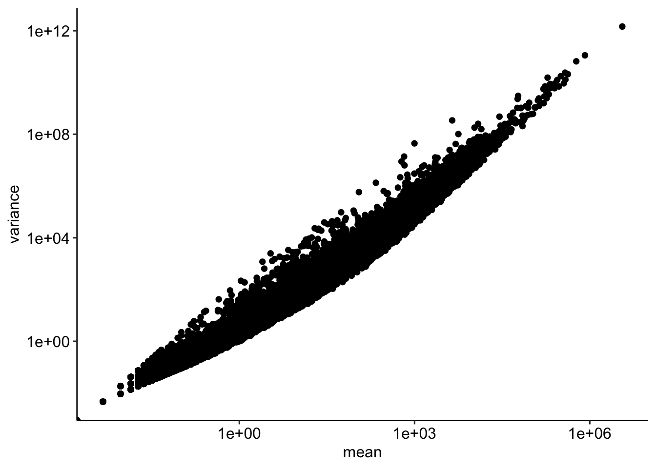
df.vsd <- data.frame(mean = rowMeans(assay(vsd)),
variance = matrixStats::rowVars(assay(vsd) %>% as.matrix()))

ggplot(df.vsd, aes(mean, variance)) + geom_point() + scale_x_log10() + scale_y_log10()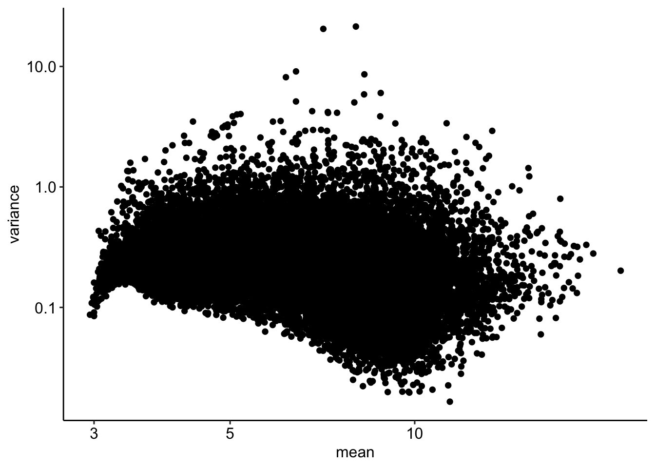
df <- data.frame(mean = log1p(rowMeans(counts)),
variance = matrixStats::rowVars(log1p( counts %>% as.matrix())))

ggplot(df, aes(mean, variance)) + geom_point() + scale_x_log10() + scale_y_log10()
Warning in scale_x_log10(): log-10 transformation introduced infinite values.Warning in scale_y_log10(): log-10 transformation introduced infinite values.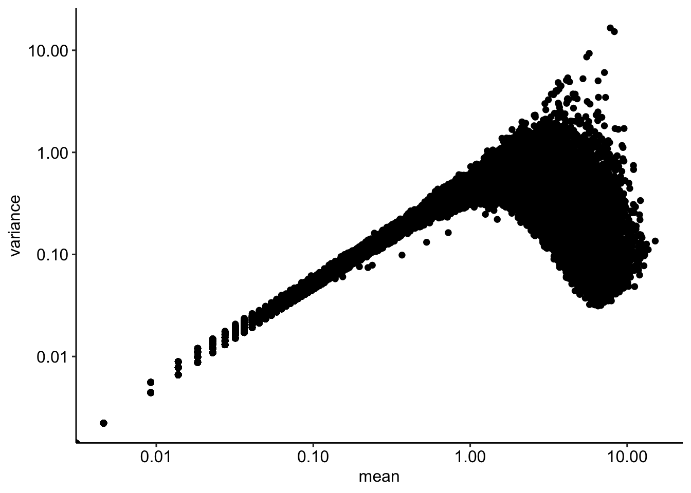
vsd$group.in.paper <- vsd$`group in paper`
plotPCA(vsd, intgroup=c('stage'))
using ntop=500 top features by varianceWarning: `aes_string()` was deprecated in ggplot2 3.0.0.
ℹ Please use tidy evaluation idioms with `aes()`.
ℹ See also `vignette("ggplot2-in-packages")` for more information.
ℹ The deprecated feature was likely used in the DESeq2 package.
Please report the issue to the authors.
What separates the clusters?
plotPCA(vsd, intgroup=c("stage"))using ntop=500 top features by variance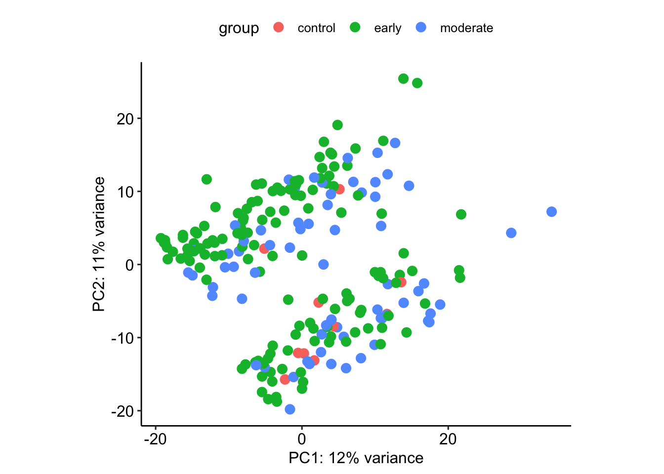
df = plotCounts(dds, gene="XIST", intgroup="sample_name", returnData = T)Warning in data.frame(count = cnts + pc, group = as.integer(group)): NAs
introduced by coerciondf count sample_name
GSM3998167 1.501596 GSM3998167
GSM3998168 7068.950701 GSM3998168
GSM3998169 4098.562347 GSM3998169
GSM3998170 0.500000 GSM3998170
GSM3998171 0.500000 GSM3998171
GSM3998172 2954.166546 GSM3998172
GSM3998173 0.500000 GSM3998173
GSM3998174 5793.053865 GSM3998174
GSM3998175 0.500000 GSM3998175
GSM3998176 0.500000 GSM3998176
GSM3998177 0.500000 GSM3998177
GSM3998178 3749.703404 GSM3998178
GSM3998179 0.500000 GSM3998179
GSM3998180 2.521483 GSM3998180
GSM3998181 1.657160 GSM3998181
GSM3998182 1.585129 GSM3998182
GSM3998183 1.620850 GSM3998183
GSM3998184 4212.240309 GSM3998184
GSM3998185 0.500000 GSM3998185
GSM3998186 4711.809688 GSM3998186
GSM3998187 5136.768643 GSM3998187
GSM3998188 0.500000 GSM3998188
GSM3998189 4565.923168 GSM3998189
GSM3998190 0.500000 GSM3998190
GSM3998191 9406.355722 GSM3998191
GSM3998192 7863.115034 GSM3998192
GSM3998193 0.500000 GSM3998193
GSM3998194 0.500000 GSM3998194
GSM3998195 6886.645271 GSM3998195
GSM3998196 0.500000 GSM3998196
GSM3998197 1.281836 GSM3998197
GSM3998198 1.946603 GSM3998198
GSM3998199 6628.930227 GSM3998199
GSM3998200 0.500000 GSM3998200
GSM3998201 1.471945 GSM3998201
GSM3998202 0.500000 GSM3998202
GSM3998203 7608.837622 GSM3998203
GSM3998204 0.500000 GSM3998204
GSM3998205 0.500000 GSM3998205
GSM3998206 8034.255274 GSM3998206
GSM3998207 8949.141467 GSM3998207
GSM3998208 7497.147344 GSM3998208
GSM3998209 9410.618405 GSM3998209
GSM3998210 4416.692733 GSM3998210
GSM3998211 4668.386837 GSM3998211
GSM3998212 0.500000 GSM3998212
GSM3998213 1.278294 GSM3998213
GSM3998214 2.626539 GSM3998214
GSM3998215 1.476825 GSM3998215
GSM3998216 4113.494764 GSM3998216
GSM3998217 10569.229676 GSM3998217
GSM3998218 9540.667460 GSM3998218
GSM3998219 1.390864 GSM3998219
GSM3998220 5016.774561 GSM3998220
GSM3998221 1.716219 GSM3998221
GSM3998222 6994.930486 GSM3998222
GSM3998223 4277.953167 GSM3998223
GSM3998224 2736.549605 GSM3998224
GSM3998225 0.500000 GSM3998225
GSM3998226 3607.775901 GSM3998226
GSM3998227 4889.920978 GSM3998227
GSM3998228 3594.411553 GSM3998228
GSM3998229 0.500000 GSM3998229
GSM3998230 0.500000 GSM3998230
GSM3998231 0.500000 GSM3998231
GSM3998232 5966.081638 GSM3998232
GSM3998233 1.384809 GSM3998233
GSM3998234 0.500000 GSM3998234
GSM3998235 0.500000 GSM3998235
GSM3998236 0.500000 GSM3998236
GSM3998237 0.500000 GSM3998237
GSM3998238 3329.198286 GSM3998238
GSM3998239 0.500000 GSM3998239
GSM3998240 4813.706751 GSM3998240
GSM3998241 4669.751495 GSM3998241
GSM3998242 0.500000 GSM3998242
GSM3998243 0.500000 GSM3998243
GSM3998244 2.565852 GSM3998244
GSM3998245 5582.495513 GSM3998245
GSM3998246 5798.716944 GSM3998246
GSM3998247 4351.056519 GSM3998247
GSM3998248 1.285942 GSM3998248
GSM3998249 9138.444433 GSM3998249
GSM3998250 1.286713 GSM3998250
GSM3998251 5561.602834 GSM3998251
GSM3998252 0.500000 GSM3998252
GSM3998253 6.110650 GSM3998253
GSM3998254 6046.856277 GSM3998254
GSM3998255 6096.463274 GSM3998255
GSM3998256 1.610302 GSM3998256
GSM3998257 7739.670553 GSM3998257
GSM3998258 6068.291980 GSM3998258
GSM3998259 0.500000 GSM3998259
GSM3998260 1.593511 GSM3998260
GSM3998261 1.454669 GSM3998261
GSM3998262 3985.905183 GSM3998262
GSM3998263 3577.952371 GSM3998263
GSM3998264 3096.430099 GSM3998264
GSM3998265 1.530379 GSM3998265
GSM3998266 3447.544604 GSM3998266
GSM3998267 2.292975 GSM3998267
GSM3998268 0.500000 GSM3998268
GSM3998269 4369.338450 GSM3998269
GSM3998270 4722.702500 GSM3998270
GSM3998271 3977.627655 GSM3998271
GSM3998272 2091.368612 GSM3998272
GSM3998273 0.500000 GSM3998273
GSM3998274 0.500000 GSM3998274
GSM3998275 0.500000 GSM3998275
GSM3998276 1689.047521 GSM3998276
GSM3998277 6439.724814 GSM3998277
GSM3998278 3838.964958 GSM3998278
GSM3998279 0.500000 GSM3998279
GSM3998280 8360.124278 GSM3998280
GSM3998281 4257.602802 GSM3998281
GSM3998282 3638.357162 GSM3998282
GSM3998283 11381.848929 GSM3998283
GSM3998284 0.500000 GSM3998284
GSM3998285 8336.690984 GSM3998285
GSM3998286 1.331327 GSM3998286
GSM3998287 0.500000 GSM3998287
GSM3998288 1.625357 GSM3998288
GSM3998289 1.526704 GSM3998289
GSM3998290 4077.387565 GSM3998290
GSM3998291 2.224217 GSM3998291
GSM3998292 2.830680 GSM3998292
GSM3998293 0.500000 GSM3998293
GSM3998294 0.500000 GSM3998294
GSM3998295 3116.156627 GSM3998295
GSM3998296 0.500000 GSM3998296
GSM3998297 0.500000 GSM3998297
GSM3998298 3709.143322 GSM3998298
GSM3998299 1.490846 GSM3998299
GSM3998300 0.500000 GSM3998300
GSM3998301 4103.240754 GSM3998301
GSM3998302 0.500000 GSM3998302
GSM3998303 0.500000 GSM3998303
GSM3998304 1.514333 GSM3998304
GSM3998305 4301.519090 GSM3998305
GSM3998306 2.623590 GSM3998306
GSM3998307 0.500000 GSM3998307
GSM3998308 6182.676597 GSM3998308
GSM3998309 0.500000 GSM3998309
GSM3998310 0.500000 GSM3998310
GSM3998311 5141.555286 GSM3998311
GSM3998312 4912.604003 GSM3998312
GSM3998313 1.369722 GSM3998313
GSM3998314 3536.690092 GSM3998314
GSM3998315 0.500000 GSM3998315
GSM3998316 1.350089 GSM3998316
GSM3998317 0.500000 GSM3998317
GSM3998318 0.500000 GSM3998318
GSM3998319 2940.098041 GSM3998319
GSM3998320 4123.895470 GSM3998320
GSM3998321 1.386462 GSM3998321
GSM3998322 1.401024 GSM3998322
GSM3998323 1.485267 GSM3998323
GSM3998324 382.459595 GSM3998324
GSM3998325 2.199589 GSM3998325
GSM3998326 0.500000 GSM3998326
GSM3998327 0.500000 GSM3998327
GSM3998328 5234.404868 GSM3998328
GSM3998329 0.500000 GSM3998329
GSM3998330 1.766977 GSM3998330
GSM3998331 0.500000 GSM3998331
GSM3998332 7965.662856 GSM3998332
GSM3998333 0.500000 GSM3998333
GSM3998334 2.008326 GSM3998334
GSM3998335 4960.778249 GSM3998335
GSM3998336 1.676476 GSM3998336
GSM3998337 0.500000 GSM3998337
GSM3998338 0.500000 GSM3998338
GSM3998339 10071.778295 GSM3998339
GSM3998340 19063.266664 GSM3998340
GSM3998341 6.871985 GSM3998341
GSM3998342 10230.603086 GSM3998342
GSM3998343 0.500000 GSM3998343
GSM3998344 0.500000 GSM3998344
GSM3998345 1738.036794 GSM3998345
GSM3998346 0.500000 GSM3998346
GSM3998347 0.500000 GSM3998347
GSM3998348 1.450098 GSM3998348
GSM3998349 4329.484904 GSM3998349
GSM3998350 0.500000 GSM3998350
GSM3998351 0.500000 GSM3998351
GSM3998352 0.500000 GSM3998352
GSM3998353 0.500000 GSM3998353
GSM3998354 2615.175536 GSM3998354
GSM3998355 5432.834786 GSM3998355
GSM3998356 2689.557113 GSM3998356
GSM3998357 2.682059 GSM3998357
GSM3998358 0.500000 GSM3998358
GSM3998359 11.957841 GSM3998359
GSM3998360 2794.894795 GSM3998360
GSM3998361 2721.143453 GSM3998361
GSM3998362 0.500000 GSM3998362
GSM3998363 3139.154393 GSM3998363
GSM3998364 0.500000 GSM3998364
GSM3998365 0.500000 GSM3998365
GSM3998366 0.500000 GSM3998366
GSM3998367 5513.488175 GSM3998367
GSM3998368 3101.980732 GSM3998368
GSM3998369 0.500000 GSM3998369
GSM3998370 6460.374064 GSM3998370
GSM3998371 3.334338 GSM3998371
GSM3998372 38.921728 GSM3998372
GSM3998373 3.377520 GSM3998373
GSM3998374 13415.231589 GSM3998374
GSM3998375 7.190631 GSM3998375
GSM3998376 6431.479791 GSM3998376
GSM3998377 1.322741 GSM3998377
GSM3998378 4805.530464 GSM3998378
GSM3998379 2.901732 GSM3998379
GSM3998380 1.443704 GSM3998380
GSM3998381 2876.000075 GSM3998381
GSM3998382 3851.618812 GSM3998382hist(df$count)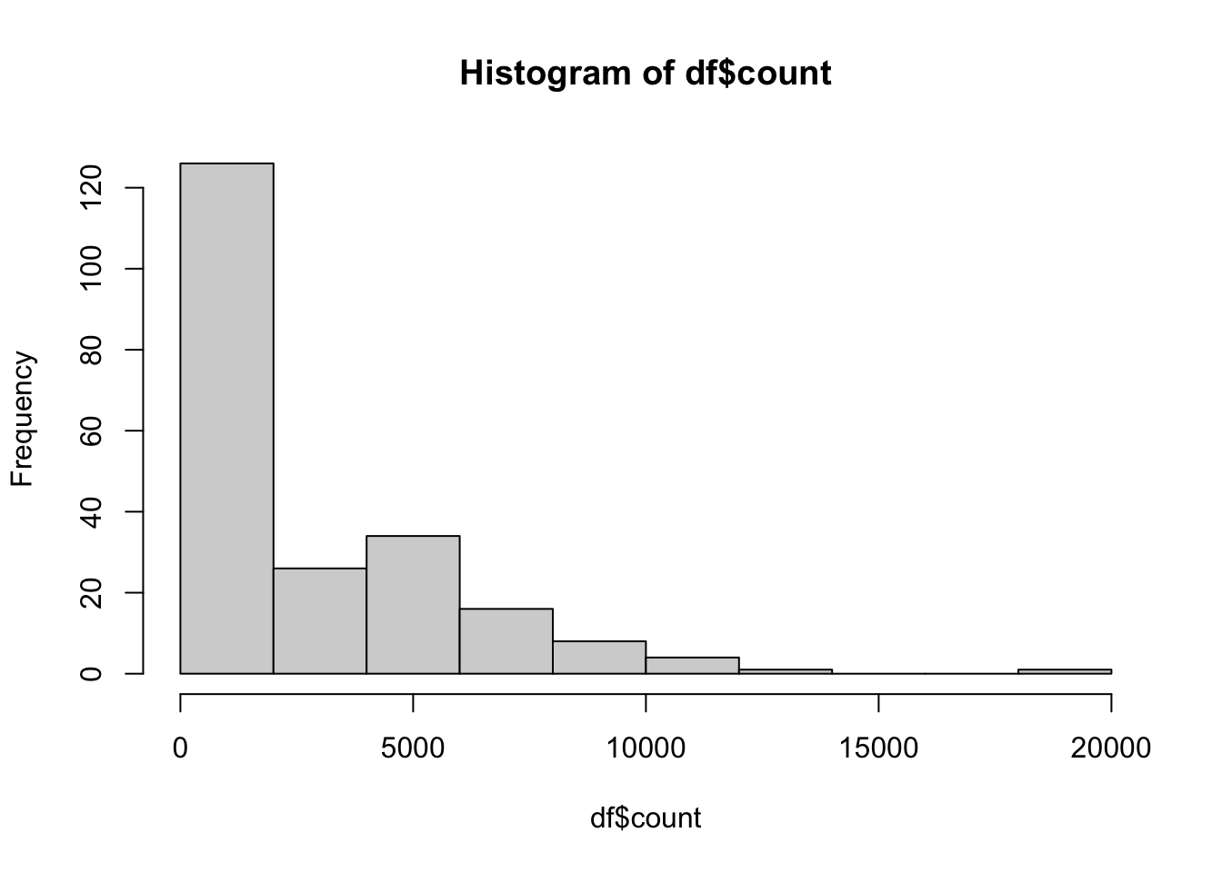
library(ggplot2)
ggplot(df, aes(count)) + stat_ecdf(geom = "point") + theme_classic(base_size = 14)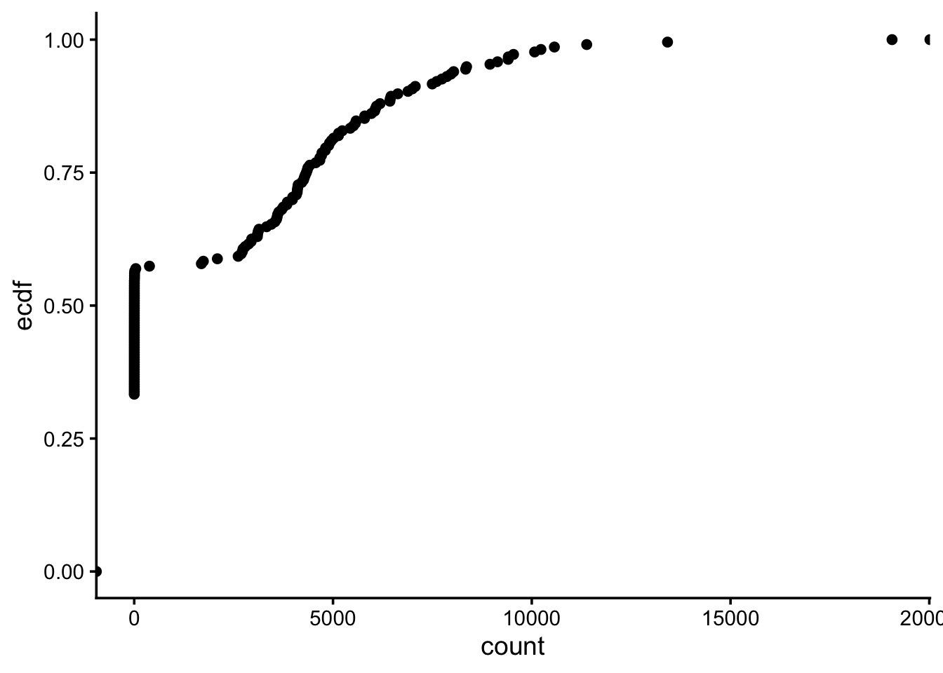
male_samples <- df[df$count<20,]$sample_namevsd$sex <- "female"
vsd$sex[vsd$sample_name %in% male_samples] <- "male"plotPCA(vsd, intgroup=c("sex"))using ntop=500 top features by variance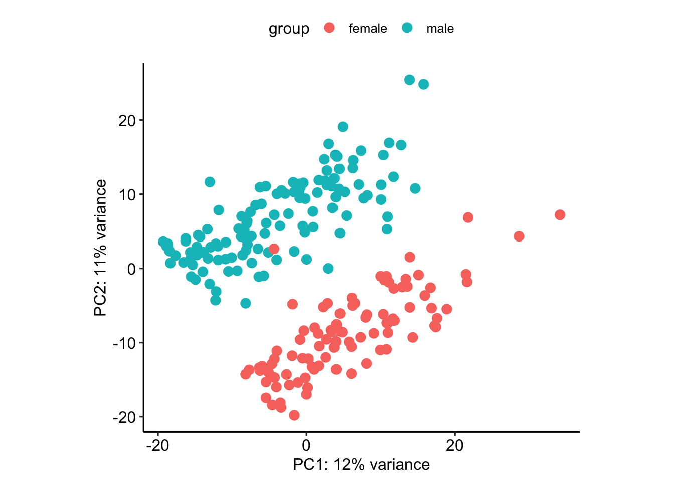
plotPCA(vsd, intgroup=c("disease"))using ntop=500 top features by variance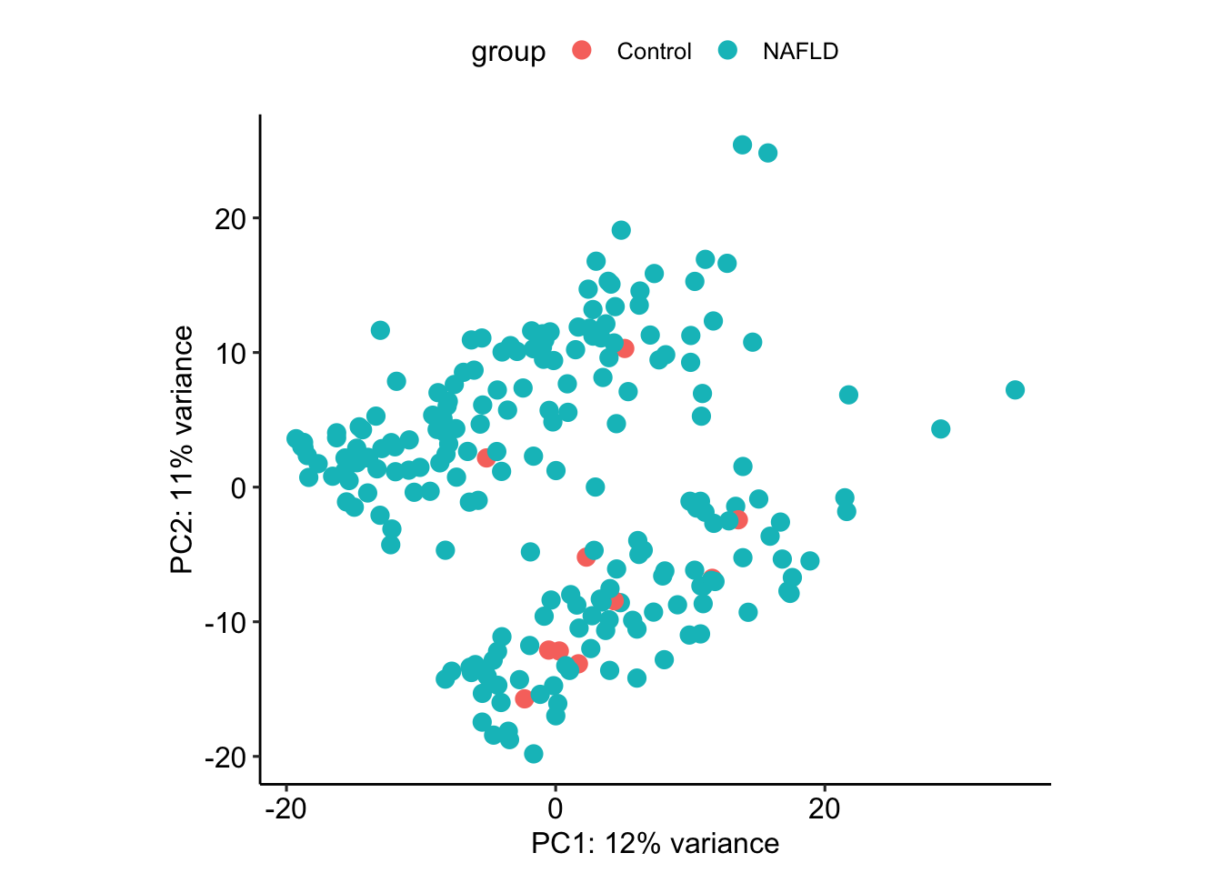
vsd.fixed <- vsd
assay(vsd.fixed) <- limma::removeBatchEffect(assay(vsd),
                                             batch=vsd$sex)
design matrix of interest not specified. Assuming a one-group experiment.plotPCA(vsd.fixed, intgroup=c("stage"))using ntop=500 top features by variance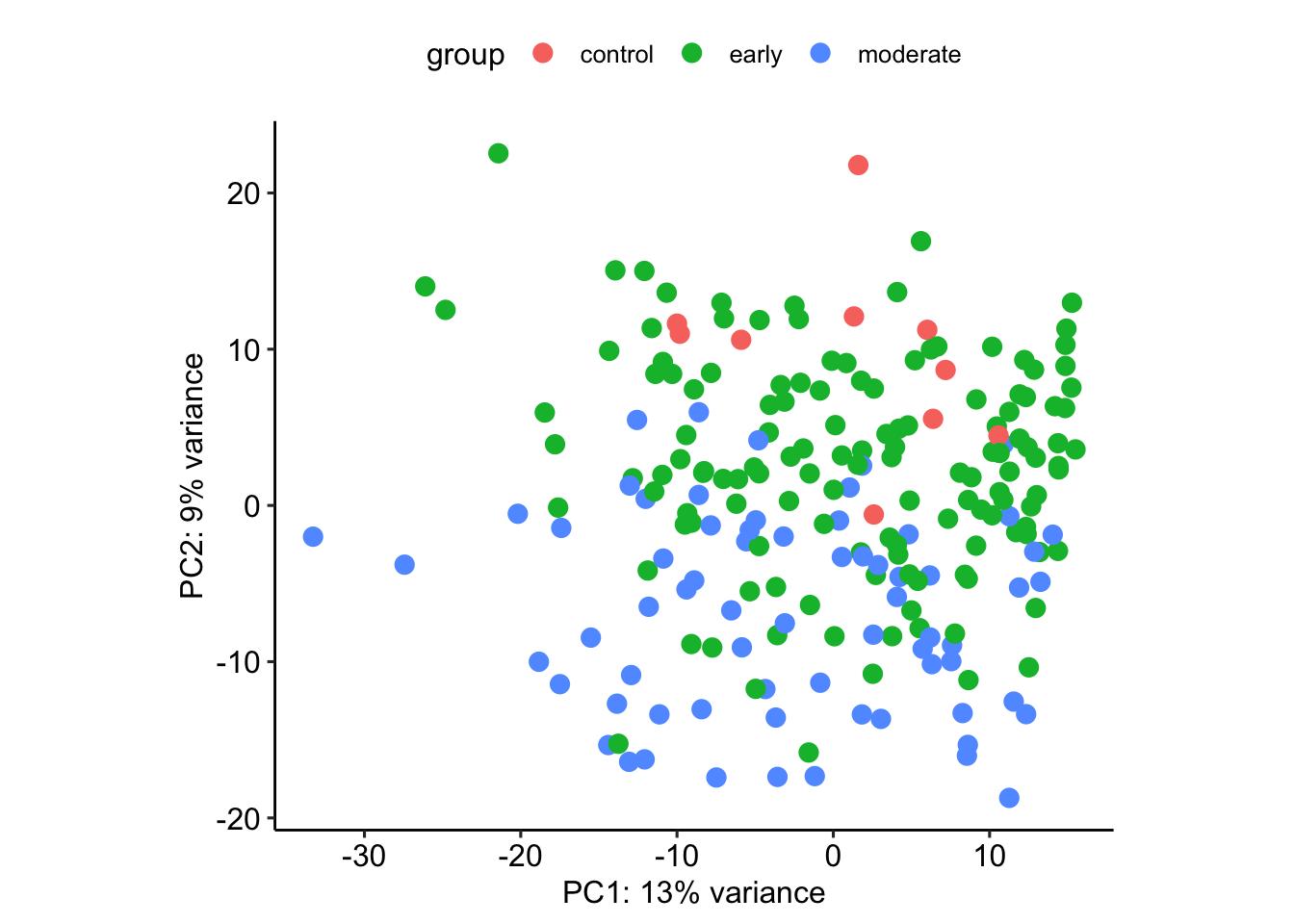
DE analsis
Let’s look at DE genes:
de_results <- results(dds,  name = "stage_early_vs_control")
de_results <- de_results %>% as.data.frame()de_results$gene <- rownames(de_results)
de_results.pos <- de_results %>% as.data.frame() %>% dplyr::filter(log2FoldChange > 1) %>% dplyr::filter(padj < 0.05)library(clusterProfiler)clusterProfiler v4.16.0 Learn more at https://yulab-smu.top/contribution-knowledge-mining/
Please cite:
G Yu. Thirteen years of clusterProfiler. The Innovation. 2024,
5(6):100722
Attaching package: 'clusterProfiler'The following object is masked from 'package:IRanges':
sliceThe following object is masked from 'package:S4Vectors':
renameThe following object is masked from 'package:purrr':
simplifyThe following object is masked from 'package:stats':
filterlibrary(org.Hs.eg.db) # install using BiocManager::install("org.Hs.eg.db")Loading required package: AnnotationDbi
Attaching package: 'AnnotationDbi'The following object is masked from 'package:clusterProfiler':
selectThe following object is masked from 'package:dplyr':
selectde.genes <- de_results.pos$gene[1:500]
universe.genes <- rownames(counts)
ego <- enrichGO(gene = de.genes,
universe = universe.genes,
OrgDb = org.Hs.eg.db,
keyType = "SYMBOL",
ont = "BP",
pAdjustMethod = "BH",
pvalueCutoff = 0.05,
qvalueCutoff = 0.05,
readable = TRUE)
head(ego) ID Description GeneRatio
GO:0008654 GO:0008654 phospholipid biosynthetic process 19/443
GO:0006739 GO:0006739 NADP metabolic process 8/443
GO:0006695 GO:0006695 cholesterol biosynthetic process 9/443
GO:1902653 GO:1902653 secondary alcohol biosynthetic process 9/443
GO:0006644 GO:0006644 phospholipid metabolic process 23/443
GO:0009743 GO:0009743 response to carbohydrate 18/443
BgRatio RichFactor FoldEnrichment zScore pvalue p.adjust
GO:0008654 239/17387 0.07949791 3.120158 5.336472 1.256437e-05 0.02663265
GO:0006739 44/17387 0.18181818 7.136056 6.589421 1.320736e-05 0.02663265
GO:0006695 65/17387 0.13846154 5.434381 5.791411 3.765528e-05 0.02920310
GO:1902653 65/17387 0.13846154 5.434381 5.791411 3.765528e-05 0.02920310
GO:0006644 354/17387 0.06497175 2.550031 4.764203 4.173743e-05 0.02920310
GO:0009743 239/17387 0.07531381 2.955939 4.923130 4.344622e-05 0.02920310
qvalue
GO:0008654 0.02418338
GO:0006739 0.02418338
GO:0006695 0.02651744
GO:1902653 0.02651744
GO:0006644 0.02651744
GO:0009743 0.02651744
geneID
GO:0008654 PIGQ/SPHK2/PITPNM2/PNPLA3/VAC14/ABCA2/CWH43/PITPNM1/MVK/HMGCS1/PIGT/ABHD8/AJUBA/PEMT/FADS1/FDPS/LIPH/PIGO/MVD
GO:0006739 FMO1/ME1/KCNAB2/GCK/TP53I3/RPTOR/FDXR/TKT
GO:0006695 CYP51A1/SREBF1/MVK/HMGCS1/APOE/TM7SF2/LSS/FDPS/MVD
GO:1902653 CYP51A1/SREBF1/MVK/HMGCS1/APOE/TM7SF2/LSS/FDPS/MVD
GO:0006644 PIGQ/SPHK2/SCARB1/PITPNM2/PNPLA3/MTMR8/VAC14/ABCA2/CWH43/PITPNM1/MVK/GPLD1/HMGCS1/PIGT/ABHD8/AJUBA/PEMT/FADS1/PLCH2/FDPS/LIPH/PIGO/MVD
GO:0009743 EXTL3/ME1/SREBF1/CMA1/TREM2/PNPLA3/OXT/GCK/COL1A1/GPLD1/SLC29A1/PDX1/RPTOR/PFKL/COL6A2/PKLR/LRP5/CDT1
Count
GO:0008654 19
GO:0006739 8
GO:0006695 9
GO:1902653 9
GO:0006644 23
GO:0009743 18barplot(ego)Warning in fortify(object, showCategory = showCategory, by = x, ...): Arguments in `...` must be used.
✖ Problematic argument:
• by = x
ℹ Did you misspell an argument name?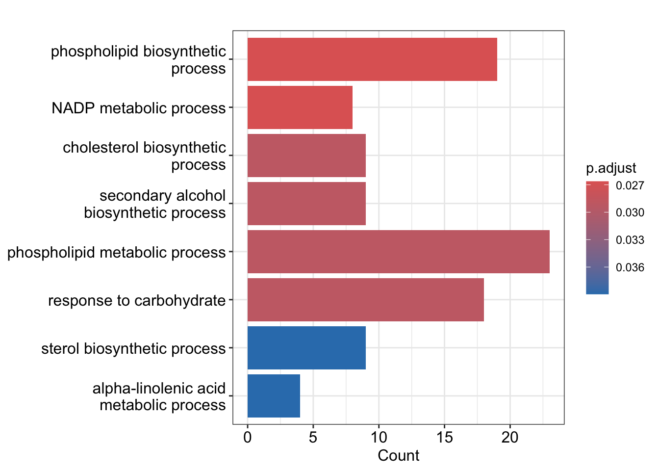
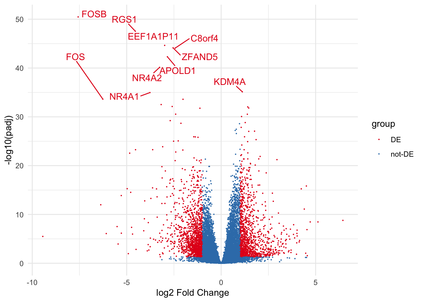
Volcano Plots
# draw volcano plot from deseq2 results
library(ggplot2)
library(ggrepel)
de_results$gene <- rownames(de_results)
de_results$gene_name <- ifelse(de_results$padj < 0.05 & abs(de_results$log2FoldChange) > 1, de_results$gene, "")
de_results$group <- ifelse(de_results$padj < 0.05 & abs(de_results$log2FoldChange) > 1, "DE", "not-DE")
de_results$size <- ifelse(de_results$padj < 0.05 & abs(de_results$log2FoldChange) > 1, 3, 1)
ggplot(de_results, aes(x = log2FoldChange, y = -log10(padj),
                       color = group)) +
    geom_point(size=0.1) +
    geom_text_repel(aes(label = gene_name), box.padding = 0.5, show.legend = F) +
    scale_color_brewer(palette = "Set1") +
    labs(x = "log2 Fold Change", y = "-log10(padj)") +
    theme_minimal()
Warning: ggrepel: 2453 unlabeled data points (too many overlaps). Consider
increasing max.overlaps