# run in terminal
wget -c --content-disposition "https://www.ncbi.nlm.nih.gov/geo/download/?acc=GS
E140511&format=file"Analysis of single=cell RNA-seq data: Signatures of Alzheimer’s
How should I run this notebook?
The easiest way to run each of the steps in this notebook is to download the raw file here, open it in Rstudio and run each code block one by one.
Biological background
Alzheimer’s disease (AD) is the most common form of dementia. Demential is a broad umbrella term for all major major neurocognitive disorders that impairs a person’s ability to remember, think, or make decisions. Pathologically, the disease is believed to occur when amyloid beta (A\(\beta\)) peptides accumulates abnormally in the extracellular space. This is followed by intraneuronal tau hyperphosphorylation and aggregation which causes neuronal and synaptic dysfunction and cell death.
The brain is made of different celltypes which can broadly be classified into three categories: excitatory, inhibitory and non-neuronal cells. Non-neuronal cells comprise of glial cells, ependymal cells, endothelial cells and pericytes. Glial cells can be further subdivided into macroglia (astrocytes and oligdendrocytes) and microglia - the primary immune cells of the central nervous system.
A number of studies have shown that among all the celltypes, microglia undergo the most prominent changes in AD brains. This is evident in two forms: 1) a change in cellular composition with AD brains exhibiting higher number of microglia and 2) a robust transcitiptional activation signal in the microglia cells. The activated microglia is referred to as DAM (Disease associated microglia) and has a distinct transcriptional signature than the homoeostatic microglia (control). This signal is conserved in mouse models (5xFAD) of AD. Multiple studies have also characterized the impact of genetic variants in the TREM2 gene. Loss of TREM2 in mice AD model (5XFAD) restricts the ability of microglia to surround A\(\beta\) plaques.
In this vignette, following Zhou et al., 2020 we will investigate the changes associated with AD pathology and TREM2 deficit brains from 5XFAD mice undergoing A\(\beta\) accumulation.
Download the object
For this vignette, we will focus on a single-cell dataset coprising 27,999 cells profiled from 15 month old mice. You can download the raw object here. For details about how the object was created see this notebook
QC steps
Downloading raw files from GEO
The raw counts matrices were deposited by authors on GEO. To download all the files, you can either download the .zip or use wget:
Quality control to discard low-quality cells
Once the files have been downloaded, we use ReadMtx to read the raw files and create one object per sample using the CreateSeuratObject function. Ultimately, we merge these objects into one object with appropriate steps for adding metadata and use the criteria defined by original authors for retaining high quality cells:
sample_names.7 <- c(
  "GSM4173504_WT_1", "GSM4173505_WT_2", "GSM4173506_WT_3",
  "GSM4173507_Trem2_KO_1", "GSM4173508_Trem2_KO_2", "GSM4173509_Trem2_KO_3",
  "GSM4173510_WT_5XFAD_1", "GSM4173511_WT_5XFAD_2", "GSM4173512_WT_5XFAD_3",
  "GSM4173513_Trem2_KO_5XFAD_1", "GSM4173514_Trem2_KO_5XFAD_2", "GSM4173515_Trem2_KO_5XFAD_3"
)

objects.list <- list()
for (sample in sample_names.7) {
  counts <- ReadMtx(
    mtx = file.path("~/github/2023_MAPS_workshop/data/Mouse_TREM2_data/", paste0(sample, "_matrix.mtx.gz")),
    cells = file.path("~/github/2023_MAPS_workshop/data/Mouse_TREM2_data/", paste0(sample, "_barcodes.tsv.gz")),
    features = file.path("~/github/2023_MAPS_workshop/data/Mouse_TREM2_data/", paste0(sample, "_features.tsv.gz"))
  )
  object <- CreateSeuratObject(counts = counts, project = sample, min.cells = 5, min.features = 5)
  object[["percent.mt"]] <- PercentageFeatureSet(object = object, pattern = "^mt-")
  object <- subset(object, nCount_RNA >= 300 & nCount_RNA < 9001 & nFeature_RNA >= 300 & nFeature_RNA < 5601 & percent.mt < 5)
  # Add a new column to the object to store the percentage of UMIs originating from mitochondrial genes (these beging with mt- such as my-Cytb)
  object[["percent.mt"]] <- PercentageFeatureSet(object = object, pattern = "^mt-")
  # Rename the cells by prefixing a sample id to make sure the cell names are unique when merging
  object <- RenameCells(object = object, add.cell.id = sample)
  object$sample_name <- sample
  objects.list[[sample]] <- object
}
object <- merge(objects.list[[1]], objects.list[2:length(objects.list)])
# 82973 samples
object$sample_name2 <- gsub(pattern = "Trem2_KO", replacement = "Trem2KO", x = object$sample_name)

object$genotype <- stringr::str_split_fixed(string = object$sample_name2, pattern = "_", n = Inf)[, 2]
object$mouse_model <- "WT"
object$mouse_model[grepl(pattern = "5XFAD", x = object$sample_name2)] <- "5XFAD"
Loading data
Before we begin, please make sure you have all the necessary packages installed. In addition to Seurat, tidyverse, ggrepel, and glmGamPoi, we will also install reshape2 and enrichR pacakges
setRepositories(ind = 1:3) # set repositories to install Bioconductor dependencies
install.packages(c("Seurat", "tidyverse", "ggrepel", "glmGamPoi", "reshape2", "org.Mm.eg.db", "org.Hs.eg.db", "clusterProfiler"))
We can read the object by providing it an appropriate path (make sure you have downloaded the object first):
suppressPackageStartupMessages({
  library(Seurat)
  library(tidyverse)
})
object <- readRDS(here::here("data/scrna/Stage15_all.rds"))
object <- JoinLayers(object)
theme_set(theme_classic(base_size = 14)) # set ggplot2 theme
Exploring the object
Before we do any downstream processing, it is always a good idea to explore the object at hand.
The counts (UMIs) are stored in the “counts” slot of the “RNA” assay”. You can read about the details of how Seurat stores its information on this wiki page.
counts <- object@assays$RNA@layers$counts
# how the first 5 gene' and first 5 cell counts
counts[1:5, 1:5]
5 x 5 sparse Matrix of class "dgCMatrix"
[1,] . . . . .
[2,] . . . . .
[3,] . . . . .
[4,] . . . . .
[5,] . . 1 . .In total we have 27999 cells (columns) and 17953 genes (rows):
dim(counts)[1] 17953 27999Among these entries, we can calculate how many proportion of entries are non-zero:
100 * round(sum(counts > 0) / (dim(counts)[1] * dim(counts)[2]), 2)[1] 4So 96% of entries in the counts matrix are zeroes (or only 4% of the values in the entire matrix are non-zeros).
# take a look at the object metadata
head(object)
orig.ident nCount_RNA nFeature_RNA
GSM4160643_WT_Cor_AAACCTGAGACCCACC-1 GSM4160643_WT_Cor 2018 708
GSM4160643_WT_Cor_AAACCTGAGAGTAAGG-1 GSM4160643_WT_Cor 952 403
GSM4160643_WT_Cor_AAACCTGAGCGATGAC-1 GSM4160643_WT_Cor 1447 769
GSM4160643_WT_Cor_AAACCTGAGTCAAGCG-1 GSM4160643_WT_Cor 1893 878
GSM4160643_WT_Cor_AAACCTGCAAAGCGGT-1 GSM4160643_WT_Cor 2023 875
GSM4160643_WT_Cor_AAACCTGCAAGCGATG-1 GSM4160643_WT_Cor 1258 746
GSM4160643_WT_Cor_AAACCTGCAAGTAGTA-1 GSM4160643_WT_Cor 1131 512
GSM4160643_WT_Cor_AAACCTGCAGTATAAG-1 GSM4160643_WT_Cor 1790 868
GSM4160643_WT_Cor_AAACCTGCATCCGTGG-1 GSM4160643_WT_Cor 1253 831
GSM4160643_WT_Cor_AAACCTGCATGCGCAC-1 GSM4160643_WT_Cor 1459 563
percent.mt sample_name
GSM4160643_WT_Cor_AAACCTGAGACCCACC-1 0.3964321 GSM4160643_WT_Cor
GSM4160643_WT_Cor_AAACCTGAGAGTAAGG-1 0.1050420 GSM4160643_WT_Cor
GSM4160643_WT_Cor_AAACCTGAGCGATGAC-1 0.5528680 GSM4160643_WT_Cor
GSM4160643_WT_Cor_AAACCTGAGTCAAGCG-1 0.4754358 GSM4160643_WT_Cor
GSM4160643_WT_Cor_AAACCTGCAAAGCGGT-1 0.1482946 GSM4160643_WT_Cor
GSM4160643_WT_Cor_AAACCTGCAAGCGATG-1 0.3974563 GSM4160643_WT_Cor
GSM4160643_WT_Cor_AAACCTGCAAGTAGTA-1 0.2652520 GSM4160643_WT_Cor
GSM4160643_WT_Cor_AAACCTGCAGTATAAG-1 0.3910615 GSM4160643_WT_Cor
GSM4160643_WT_Cor_AAACCTGCATCCGTGG-1 4.5490822 GSM4160643_WT_Cor
GSM4160643_WT_Cor_AAACCTGCATGCGCAC-1 1.3022618 GSM4160643_WT_Cor
sample_name2 genotype region
GSM4160643_WT_Cor_AAACCTGAGACCCACC-1 GSM4160643_WT_Cor WT Cortex
GSM4160643_WT_Cor_AAACCTGAGAGTAAGG-1 GSM4160643_WT_Cor WT Cortex
GSM4160643_WT_Cor_AAACCTGAGCGATGAC-1 GSM4160643_WT_Cor WT Cortex
GSM4160643_WT_Cor_AAACCTGAGTCAAGCG-1 GSM4160643_WT_Cor WT Cortex
GSM4160643_WT_Cor_AAACCTGCAAAGCGGT-1 GSM4160643_WT_Cor WT Cortex
GSM4160643_WT_Cor_AAACCTGCAAGCGATG-1 GSM4160643_WT_Cor WT Cortex
GSM4160643_WT_Cor_AAACCTGCAAGTAGTA-1 GSM4160643_WT_Cor WT Cortex
GSM4160643_WT_Cor_AAACCTGCAGTATAAG-1 GSM4160643_WT_Cor WT Cortex
GSM4160643_WT_Cor_AAACCTGCATCCGTGG-1 GSM4160643_WT_Cor WT Cortex
GSM4160643_WT_Cor_AAACCTGCATGCGCAC-1 GSM4160643_WT_Cor WT Cortex
mouse_model
GSM4160643_WT_Cor_AAACCTGAGACCCACC-1 WT
GSM4160643_WT_Cor_AAACCTGAGAGTAAGG-1 WT
GSM4160643_WT_Cor_AAACCTGAGCGATGAC-1 WT
GSM4160643_WT_Cor_AAACCTGAGTCAAGCG-1 WT
GSM4160643_WT_Cor_AAACCTGCAAAGCGGT-1 WT
GSM4160643_WT_Cor_AAACCTGCAAGCGATG-1 WT
GSM4160643_WT_Cor_AAACCTGCAAGTAGTA-1 WT
GSM4160643_WT_Cor_AAACCTGCAGTATAAG-1 WT
GSM4160643_WT_Cor_AAACCTGCATCCGTGG-1 WT
GSM4160643_WT_Cor_AAACCTGCATGCGCAC-1 WTYou can add a custom column to the metadata using:
# add a new metadata column
object$my_column <- "test"
head(object)
orig.ident nCount_RNA nFeature_RNA
GSM4160643_WT_Cor_AAACCTGAGACCCACC-1 GSM4160643_WT_Cor 2018 708
GSM4160643_WT_Cor_AAACCTGAGAGTAAGG-1 GSM4160643_WT_Cor 952 403
GSM4160643_WT_Cor_AAACCTGAGCGATGAC-1 GSM4160643_WT_Cor 1447 769
GSM4160643_WT_Cor_AAACCTGAGTCAAGCG-1 GSM4160643_WT_Cor 1893 878
GSM4160643_WT_Cor_AAACCTGCAAAGCGGT-1 GSM4160643_WT_Cor 2023 875
GSM4160643_WT_Cor_AAACCTGCAAGCGATG-1 GSM4160643_WT_Cor 1258 746
GSM4160643_WT_Cor_AAACCTGCAAGTAGTA-1 GSM4160643_WT_Cor 1131 512
GSM4160643_WT_Cor_AAACCTGCAGTATAAG-1 GSM4160643_WT_Cor 1790 868
GSM4160643_WT_Cor_AAACCTGCATCCGTGG-1 GSM4160643_WT_Cor 1253 831
GSM4160643_WT_Cor_AAACCTGCATGCGCAC-1 GSM4160643_WT_Cor 1459 563
percent.mt sample_name
GSM4160643_WT_Cor_AAACCTGAGACCCACC-1 0.3964321 GSM4160643_WT_Cor
GSM4160643_WT_Cor_AAACCTGAGAGTAAGG-1 0.1050420 GSM4160643_WT_Cor
GSM4160643_WT_Cor_AAACCTGAGCGATGAC-1 0.5528680 GSM4160643_WT_Cor
GSM4160643_WT_Cor_AAACCTGAGTCAAGCG-1 0.4754358 GSM4160643_WT_Cor
GSM4160643_WT_Cor_AAACCTGCAAAGCGGT-1 0.1482946 GSM4160643_WT_Cor
GSM4160643_WT_Cor_AAACCTGCAAGCGATG-1 0.3974563 GSM4160643_WT_Cor
GSM4160643_WT_Cor_AAACCTGCAAGTAGTA-1 0.2652520 GSM4160643_WT_Cor
GSM4160643_WT_Cor_AAACCTGCAGTATAAG-1 0.3910615 GSM4160643_WT_Cor
GSM4160643_WT_Cor_AAACCTGCATCCGTGG-1 4.5490822 GSM4160643_WT_Cor
GSM4160643_WT_Cor_AAACCTGCATGCGCAC-1 1.3022618 GSM4160643_WT_Cor
sample_name2 genotype region
GSM4160643_WT_Cor_AAACCTGAGACCCACC-1 GSM4160643_WT_Cor WT Cortex
GSM4160643_WT_Cor_AAACCTGAGAGTAAGG-1 GSM4160643_WT_Cor WT Cortex
GSM4160643_WT_Cor_AAACCTGAGCGATGAC-1 GSM4160643_WT_Cor WT Cortex
GSM4160643_WT_Cor_AAACCTGAGTCAAGCG-1 GSM4160643_WT_Cor WT Cortex
GSM4160643_WT_Cor_AAACCTGCAAAGCGGT-1 GSM4160643_WT_Cor WT Cortex
GSM4160643_WT_Cor_AAACCTGCAAGCGATG-1 GSM4160643_WT_Cor WT Cortex
GSM4160643_WT_Cor_AAACCTGCAAGTAGTA-1 GSM4160643_WT_Cor WT Cortex
GSM4160643_WT_Cor_AAACCTGCAGTATAAG-1 GSM4160643_WT_Cor WT Cortex
GSM4160643_WT_Cor_AAACCTGCATCCGTGG-1 GSM4160643_WT_Cor WT Cortex
GSM4160643_WT_Cor_AAACCTGCATGCGCAC-1 GSM4160643_WT_Cor WT Cortex
mouse_model my_column
GSM4160643_WT_Cor_AAACCTGAGACCCACC-1 WT test
GSM4160643_WT_Cor_AAACCTGAGAGTAAGG-1 WT test
GSM4160643_WT_Cor_AAACCTGAGCGATGAC-1 WT test
GSM4160643_WT_Cor_AAACCTGAGTCAAGCG-1 WT test
GSM4160643_WT_Cor_AAACCTGCAAAGCGGT-1 WT test
GSM4160643_WT_Cor_AAACCTGCAAGCGATG-1 WT test
GSM4160643_WT_Cor_AAACCTGCAAGTAGTA-1 WT test
GSM4160643_WT_Cor_AAACCTGCAGTATAAG-1 WT test
GSM4160643_WT_Cor_AAACCTGCATCCGTGG-1 WT test
GSM4160643_WT_Cor_AAACCTGCATGCGCAC-1 WT testOr delete the column from the metadata:
object$my_column <- NULL
head(object)
orig.ident nCount_RNA nFeature_RNA
GSM4160643_WT_Cor_AAACCTGAGACCCACC-1 GSM4160643_WT_Cor 2018 708
GSM4160643_WT_Cor_AAACCTGAGAGTAAGG-1 GSM4160643_WT_Cor 952 403
GSM4160643_WT_Cor_AAACCTGAGCGATGAC-1 GSM4160643_WT_Cor 1447 769
GSM4160643_WT_Cor_AAACCTGAGTCAAGCG-1 GSM4160643_WT_Cor 1893 878
GSM4160643_WT_Cor_AAACCTGCAAAGCGGT-1 GSM4160643_WT_Cor 2023 875
GSM4160643_WT_Cor_AAACCTGCAAGCGATG-1 GSM4160643_WT_Cor 1258 746
GSM4160643_WT_Cor_AAACCTGCAAGTAGTA-1 GSM4160643_WT_Cor 1131 512
GSM4160643_WT_Cor_AAACCTGCAGTATAAG-1 GSM4160643_WT_Cor 1790 868
GSM4160643_WT_Cor_AAACCTGCATCCGTGG-1 GSM4160643_WT_Cor 1253 831
GSM4160643_WT_Cor_AAACCTGCATGCGCAC-1 GSM4160643_WT_Cor 1459 563
percent.mt sample_name
GSM4160643_WT_Cor_AAACCTGAGACCCACC-1 0.3964321 GSM4160643_WT_Cor
GSM4160643_WT_Cor_AAACCTGAGAGTAAGG-1 0.1050420 GSM4160643_WT_Cor
GSM4160643_WT_Cor_AAACCTGAGCGATGAC-1 0.5528680 GSM4160643_WT_Cor
GSM4160643_WT_Cor_AAACCTGAGTCAAGCG-1 0.4754358 GSM4160643_WT_Cor
GSM4160643_WT_Cor_AAACCTGCAAAGCGGT-1 0.1482946 GSM4160643_WT_Cor
GSM4160643_WT_Cor_AAACCTGCAAGCGATG-1 0.3974563 GSM4160643_WT_Cor
GSM4160643_WT_Cor_AAACCTGCAAGTAGTA-1 0.2652520 GSM4160643_WT_Cor
GSM4160643_WT_Cor_AAACCTGCAGTATAAG-1 0.3910615 GSM4160643_WT_Cor
GSM4160643_WT_Cor_AAACCTGCATCCGTGG-1 4.5490822 GSM4160643_WT_Cor
GSM4160643_WT_Cor_AAACCTGCATGCGCAC-1 1.3022618 GSM4160643_WT_Cor
sample_name2 genotype region
GSM4160643_WT_Cor_AAACCTGAGACCCACC-1 GSM4160643_WT_Cor WT Cortex
GSM4160643_WT_Cor_AAACCTGAGAGTAAGG-1 GSM4160643_WT_Cor WT Cortex
GSM4160643_WT_Cor_AAACCTGAGCGATGAC-1 GSM4160643_WT_Cor WT Cortex
GSM4160643_WT_Cor_AAACCTGAGTCAAGCG-1 GSM4160643_WT_Cor WT Cortex
GSM4160643_WT_Cor_AAACCTGCAAAGCGGT-1 GSM4160643_WT_Cor WT Cortex
GSM4160643_WT_Cor_AAACCTGCAAGCGATG-1 GSM4160643_WT_Cor WT Cortex
GSM4160643_WT_Cor_AAACCTGCAAGTAGTA-1 GSM4160643_WT_Cor WT Cortex
GSM4160643_WT_Cor_AAACCTGCAGTATAAG-1 GSM4160643_WT_Cor WT Cortex
GSM4160643_WT_Cor_AAACCTGCATCCGTGG-1 GSM4160643_WT_Cor WT Cortex
GSM4160643_WT_Cor_AAACCTGCATGCGCAC-1 GSM4160643_WT_Cor WT Cortex
mouse_model
GSM4160643_WT_Cor_AAACCTGAGACCCACC-1 WT
GSM4160643_WT_Cor_AAACCTGAGAGTAAGG-1 WT
GSM4160643_WT_Cor_AAACCTGAGCGATGAC-1 WT
GSM4160643_WT_Cor_AAACCTGAGTCAAGCG-1 WT
GSM4160643_WT_Cor_AAACCTGCAAAGCGGT-1 WT
GSM4160643_WT_Cor_AAACCTGCAAGCGATG-1 WT
GSM4160643_WT_Cor_AAACCTGCAAGTAGTA-1 WT
GSM4160643_WT_Cor_AAACCTGCAGTATAAG-1 WT
GSM4160643_WT_Cor_AAACCTGCATCCGTGG-1 WT
GSM4160643_WT_Cor_AAACCTGCATGCGCAC-1 WTYou can plot some QC metrics using the VlnPlot command:
VlnPlot(object, features = c("nCount_RNA", "nFeature_RNA", "percent.mt"))Warning: Default search for "data" layer in "RNA" assay yielded no results;
utilizing "counts" layer instead.Warning: The `slot` argument of `FetchData()` is deprecated as of SeuratObject 5.0.0.
ℹ Please use the `layer` argument instead.
ℹ The deprecated feature was likely used in the Seurat package.
Please report the issue at <https://github.com/satijalab/seurat/issues>.Warning: `PackageCheck()` was deprecated in SeuratObject 5.0.0.
ℹ Please use `rlang::check_installed()` instead.
ℹ The deprecated feature was likely used in the Seurat package.
Please report the issue at <https://github.com/satijalab/seurat/issues>.Warning: `aes_string()` was deprecated in ggplot2 3.0.0.
ℹ Please use tidy evaluation idioms with `aes()`.
ℹ See also `vignette("ggplot2-in-packages")` for more information.
ℹ The deprecated feature was likely used in the Seurat package.
Please report the issue at <https://github.com/satijalab/seurat/issues>.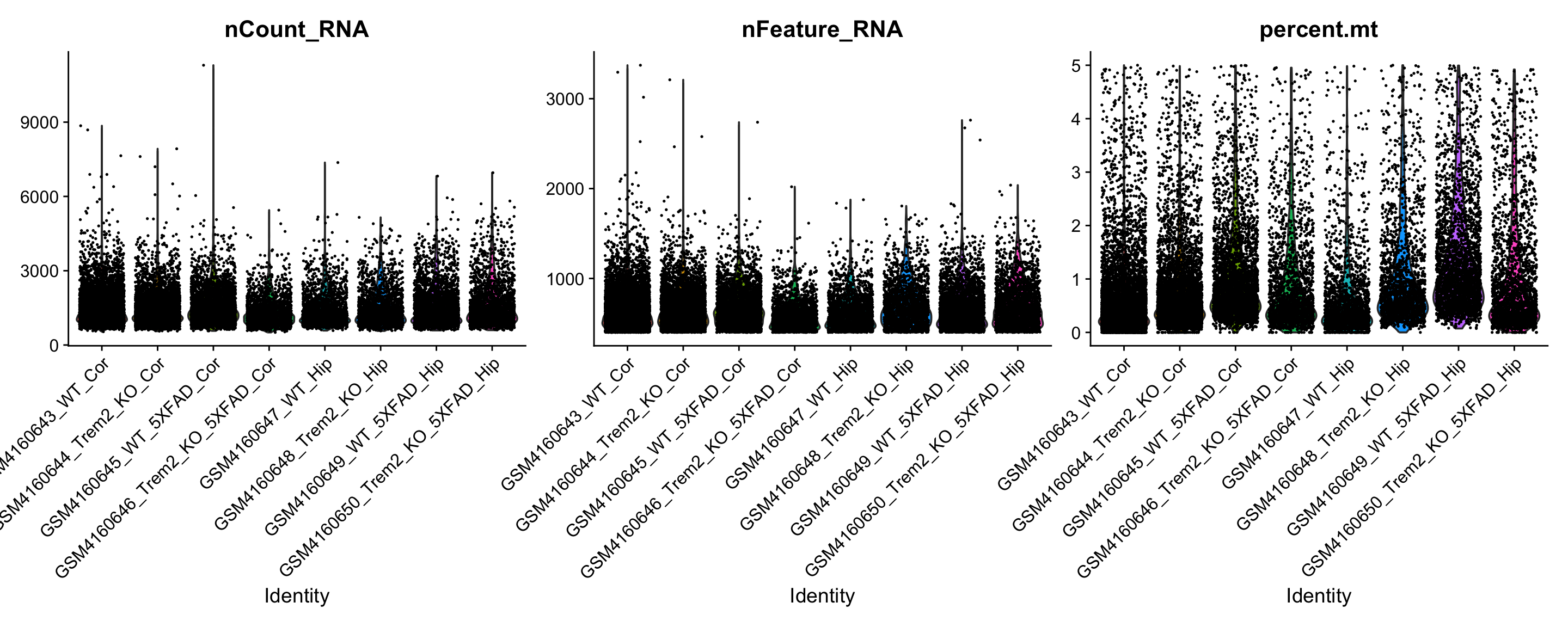
You can see the help associated with this (or any function) function by typing ‘?VlnPlot’ in the RStudio console.
Feature Selection
Many genes in this dataset are “not informative” - they are either lowly expressed overall, or expressed in all the celltypes. For downstream analysis, we want to identify “informative” genes - this increases the signal to noise ratio for downstream dimensionaloty reduction.
One way to select these genes would be to calculate a per-gene variance and select the ones with the highest variance. Let’s explore the mean-variance relationship of these genes:
# get UMI counts from object
counts <- GetAssayData(object = object, assay = "RNA", slot = "counts")
Warning: The `slot` argument of `GetAssayData()` is deprecated as of SeuratObject 5.0.0.
ℹ Please use the `layer` argument instead.# calculate per gene mean
gene_mean <- rowMeans(x = counts)
gene_variance <- apply(X = counts, MARGIN = 1, FUN = var)Warning in asMethod(object): sparse->dense coercion: allocating vector of size
3.7 GiBggplot(data = data.frame("gene_mean" = gene_mean, "gene_variance" = gene_variance), aes(gene_mean, gene_variance)) +
geom_point() +
geom_abline(color="red")+
scale_x_log10() +
scale_y_log10() +
xlab("Gene mean") +
ylab("Gene variance") +
theme_bw(base_size = 14) Warning in scale_x_log10(): log-10 transformation introduced infinite values.Warning in scale_y_log10(): log-10 transformation introduced infinite values.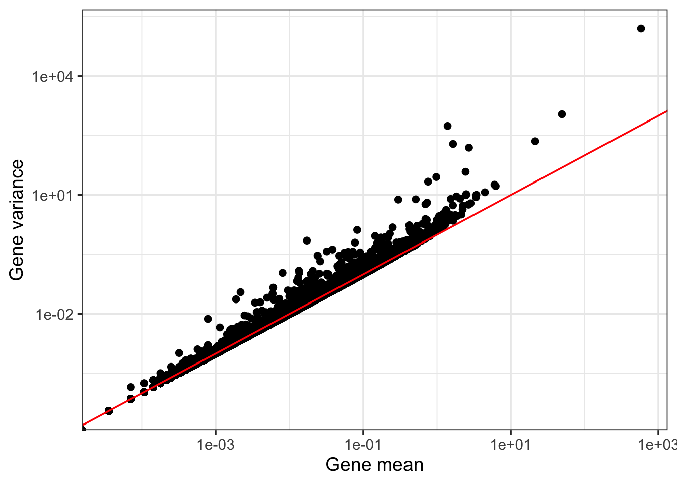
So genes with higher means will also have higher variance because there is a strong mean-variance relationship exhibited by all genes. One way to adjust for this relationship is to explicitly model the mean-variance relationship by fitting a smooth curve and then identify genes that show high deviation from this “expected” pattern. This is essentially what is done inside the FindVariableFeatures function:
object <- FindVariableFeatures(object = object, selection.method = "vst")Finding variable features for layer countsVariableFeaturePlot(object)Warning in scale_x_log10(): log-10 transformation introduced infinite values.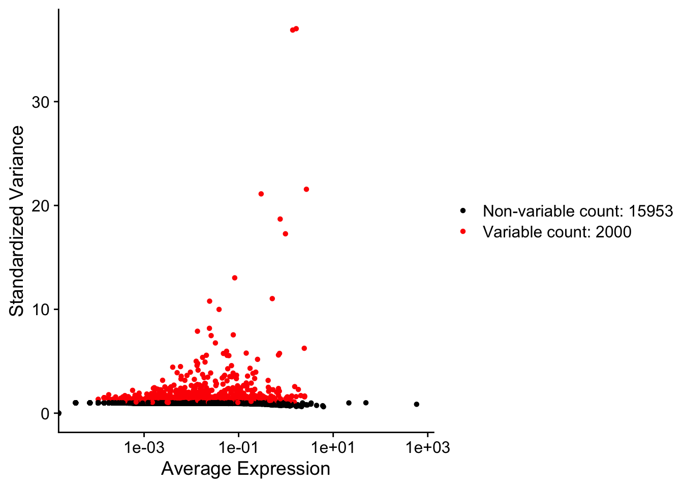
In the plot above, the “variable genes” are highlhted in red and as clear from their mean values are not necessarily the most highly expressed (notice the genes with average expression > 10)
Normalization
The total number of UMIs observed for a cell are attributable to 1) cell size (higher cell size => more RNA content => more expected UMIs) and 2) sequencing depth. Let’s look at the expression of a ubiquoulsy expressed gene (Malat1- a long noncoding RNA):
total_umis <- colSums(x = counts)
gene <- "Malat1"
gene_umi <- as.numeric(counts[gene, ])

ggplot(data = data.frame("total_cell_umi" = total_umis, "gene_umi" = gene_umi), aes(total_cell_umi, gene_umi)) +
  geom_point() +
  theme_bw(base_size = 14) + xlab("Total sequencing depth") + ylab(paste0("Gene UMI(", gene))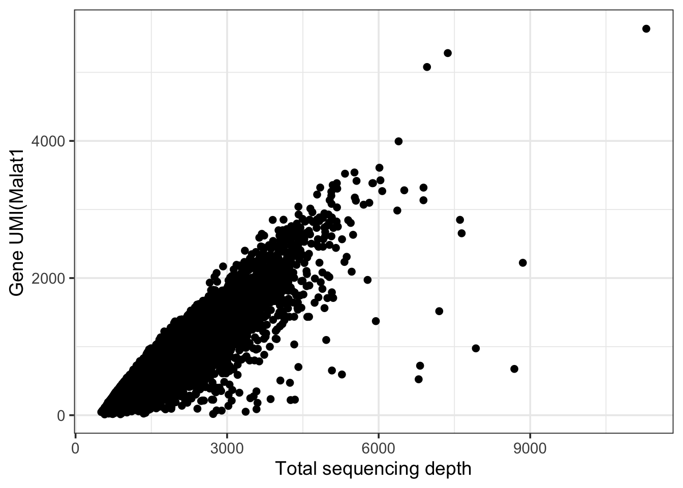
This gene (Malat1) shows an almost linear relationship with sequencing depth of a cell. In this case the “heterogeneity across cells” in expression levels of Malat1 are primarly attributable to the fact that these cells were sequenced to different deths and is un interesting.
If all the genes showed this linear behavior we could have simply “regressed” out the effect of sequencing depth by performing a linear regression of observed gene count agaisnt the total sequencing depth of the cell. But it is not a good idea because there are also marker genes such as Apoe (an astrocytes marker), Vip (a marker for Vip interneurons - these are a type of inhibitory neurons) and C1qa (a marker of microglia)
data.to.plot <- FetchData(object = object, slot = "counts", vars = c("Apoe", "Vip", "C1qa", "nCount_RNA"))
head(data.to.plot)
Apoe Vip C1qa nCount_RNA
GSM4160643_WT_Cor_AAACCTGAGACCCACC-1 0 0 0 2018
GSM4160643_WT_Cor_AAACCTGAGAGTAAGG-1 0 0 0 952
GSM4160643_WT_Cor_AAACCTGAGCGATGAC-1 0 0 0 1447
GSM4160643_WT_Cor_AAACCTGAGTCAAGCG-1 0 0 0 1893
GSM4160643_WT_Cor_AAACCTGCAAAGCGGT-1 0 0 1 2023
GSM4160643_WT_Cor_AAACCTGCAAGCGATG-1 0 0 0 1258data.to.plot.genewise <- reshape2::melt(data.to.plot, id.vars = "nCount_RNA")
ggplot(data.to.plot.genewise, aes(nCount_RNA, value)) +
geom_point() +
facet_wrap(~variable) +
xlab("Sequencing depth") +
ylab("Gene UMI") +
theme_bw(base_size = 14)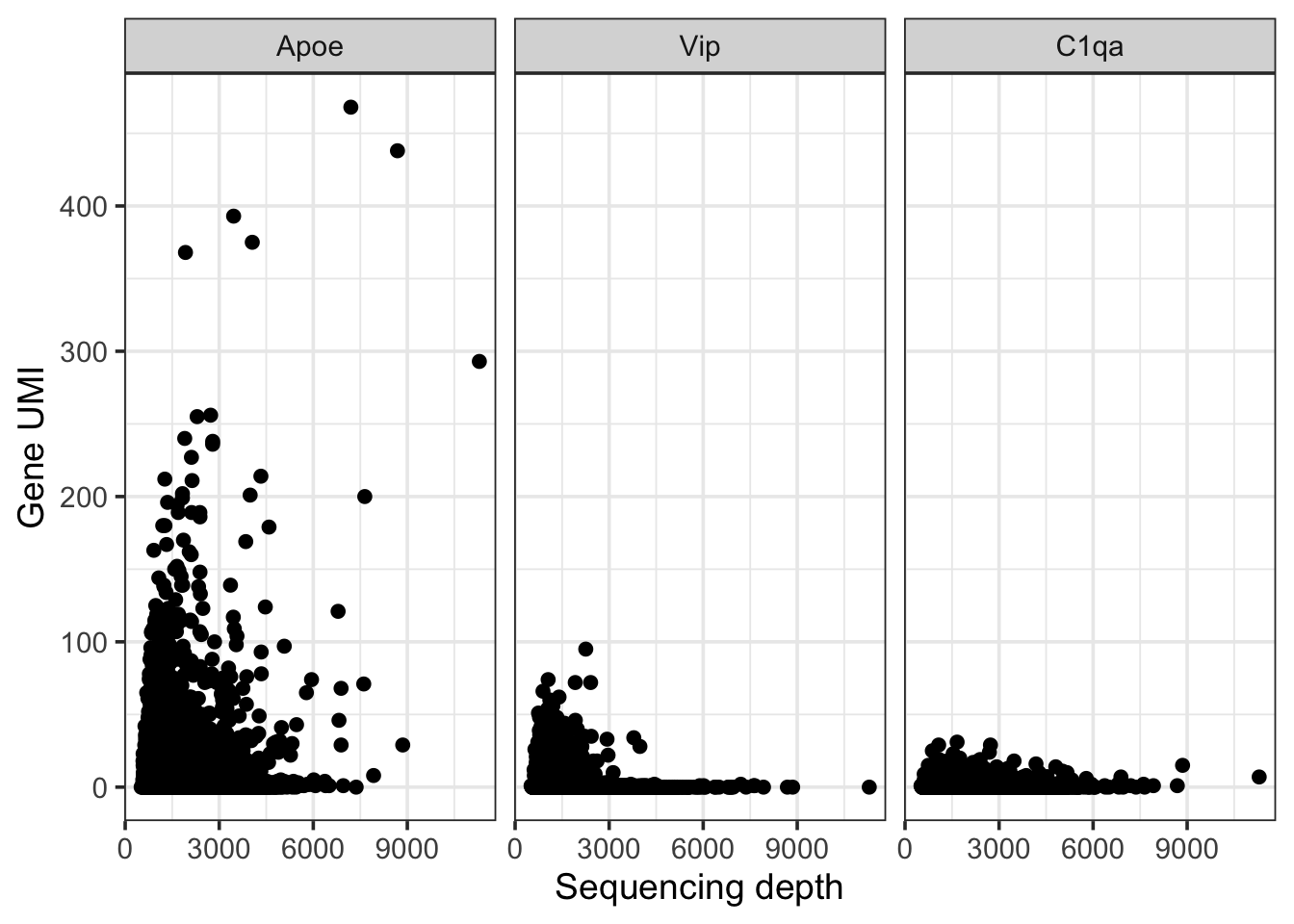
Given these are marker genes, they are only expressed in a subset of cells. A simple linear regression where we regress out the sequencing depth from each gene’s UMI will end up affecting these marker genes negatively - dampening their expression.
Log Normalization
Instead of regressing out sequencing depth, an alternate idea is to to use a global scale factor (say 10,000) and “scale” all cells to have this sequencing depth while also accounting for the sequencing depth of the cell. To reduce the impact of outliers, these scaled values are log transformed (after adding a pseudocount of 1). To perform this normalizing using Seurat, you can use the NormalizeData function:
object <- NormalizeData(object = object, scale.factor = 10000)Normalizing layer: countsWhat is “good normalization”?
There are two key properties that any “good normalization” method should achieve:
The normalized expression values of a gene should have minimal dependence on the seuquencing depth
The variance of normalized gene expression values across should cells should primarily reflect biological variation and not technical noise and should be independent of gene’s mean expression level or sequencing depth of the cell.
Let’s look into the expression pattern of the same highly expressed gene after running Log Normalization:
gene <- "Malat1"
# normalized values are stored in the "data" slot
object <- NormalizeData(object = object, scale.factor = 10000)
Normalizing layer: countslognormalized.data <- GetAssayData(object = object, assay = "RNA", slot = "data")[gene, ]
ggplot(data.frame("sequencing_depth" = colSums(x = counts), "normalized_values" = lognormalized.data), aes(sequencing_depth, normalized_values)) +
geom_point() +
theme_bw(base_size = 14)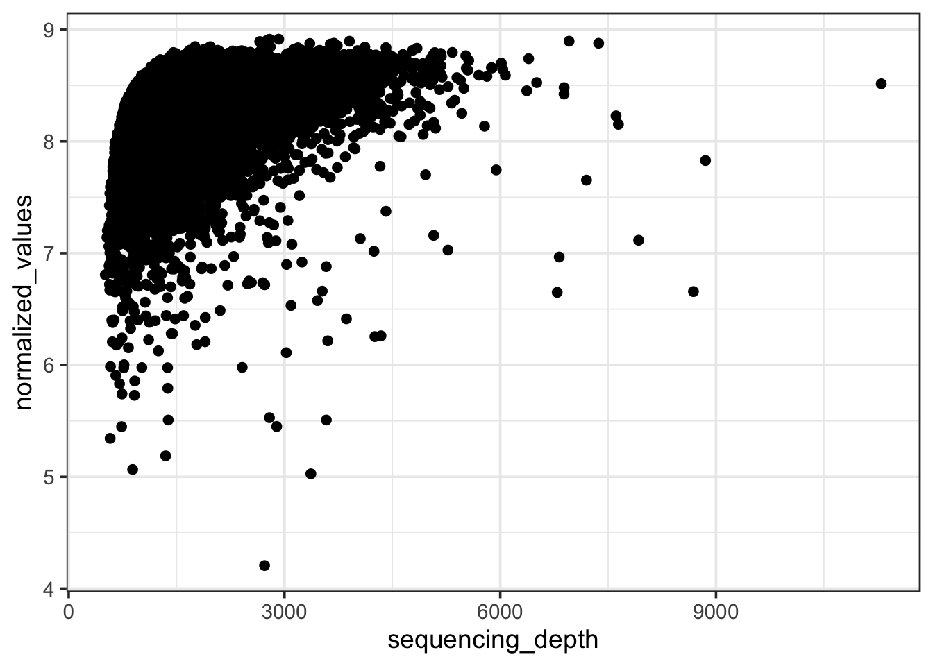
Compare this relationship with an earlier figure where we were plotting the raw expression values - the correlation between y and x axis has reduced significantly. But as we will see in the next figure, this correlation is not zero.
counts <- GetAssayData(object = object, assay = "RNA", slot = "counts")
lognormalized.data <- GetAssayData(object = object, assay = "RNA", slot = "data")

# compute per gene correlation with sequencing depth of each cell
var.features <- VariableFeatures(object = object)

corr.counts <- apply(X = counts[var.features, ], MARGIN = 1, FUN = function(x) cor(x = x, y = colSums(x = counts)))
corr.lognorm <- apply(X = lognormalized.data[var.features, ], MARGIN = 1, FUN = function(x) cor(x = x, y = colSums(x = counts)))

df <- data.frame(corr = c(corr.counts, corr.lognorm), type = c(
  rep("Raw counts", length(corr.counts)),
  rep("Log normalized", length(corr.lognorm))
))

ggplot(data = df, aes(corr, fill = type)) +
  geom_histogram() +
  theme_bw(base_size = 14)
`stat_bin()` using `bins = 30`. Pick better value `binwidth`.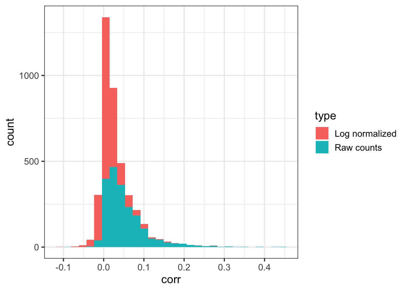
One step normalization and feature selection: SCTransform
A second way to achieve variance stabilization (and variable feature selection) is by using SCTransform. In SCTransform, we use a regularized negative binomial model to directly model the single-cell counts. The normalized counts are then cacluclated by reversing this general reltaionship by substituting the observed count depth as the median sequencing depth. You can read the SCTransform publication for more details (SCTransform SCTransform-v2).
We will use SCTransform based analysis for the rest of the work flow.
object <- SCTransform(object = object,
                      vst.flavor = "v2", verbose = FALSE)
Warning: The `slot` argument of `SetAssayData()` is deprecated as of SeuratObject 5.0.0.
ℹ Please use the `layer` argument instead.
ℹ The deprecated feature was likely used in the Seurat package.
Please report the issue at <https://github.com/satijalab/seurat/issues>.Compare the correlation of SCT normalized data with sequencing depth:
sct.data <- GetAssayData(object = object, assay = "SCT", slot = "data")
corr.sct <- apply(X = sct.data[intersect(var.features, rownames(sct.data)), ], MARGIN = 1, FUN = function(x) cor(x = x, y = colSums(x = counts)))
Warning in cor(x = x, y = colSums(x = counts)): the standard deviation is zero
Warning in cor(x = x, y = colSums(x = counts)): the standard deviation is zero
Warning in cor(x = x, y = colSums(x = counts)): the standard deviation is zero
Warning in cor(x = x, y = colSums(x = counts)): the standard deviation is zero
Warning in cor(x = x, y = colSums(x = counts)): the standard deviation is zero
Warning in cor(x = x, y = colSums(x = counts)): the standard deviation is zero
Warning in cor(x = x, y = colSums(x = counts)): the standard deviation is zero
Warning in cor(x = x, y = colSums(x = counts)): the standard deviation is zero
Warning in cor(x = x, y = colSums(x = counts)): the standard deviation is zero
Warning in cor(x = x, y = colSums(x = counts)): the standard deviation is zero
Warning in cor(x = x, y = colSums(x = counts)): the standard deviation is zero
Warning in cor(x = x, y = colSums(x = counts)): the standard deviation is zero
Warning in cor(x = x, y = colSums(x = counts)): the standard deviation is zero
Warning in cor(x = x, y = colSums(x = counts)): the standard deviation is zero
Warning in cor(x = x, y = colSums(x = counts)): the standard deviation is zero
Warning in cor(x = x, y = colSums(x = counts)): the standard deviation is zero
Warning in cor(x = x, y = colSums(x = counts)): the standard deviation is zero
Warning in cor(x = x, y = colSums(x = counts)): the standard deviation is zero
Warning in cor(x = x, y = colSums(x = counts)): the standard deviation is zero
Warning in cor(x = x, y = colSums(x = counts)): the standard deviation is zero
Warning in cor(x = x, y = colSums(x = counts)): the standard deviation is zero
Warning in cor(x = x, y = colSums(x = counts)): the standard deviation is zero
Warning in cor(x = x, y = colSums(x = counts)): the standard deviation is zero
Warning in cor(x = x, y = colSums(x = counts)): the standard deviation is zero
Warning in cor(x = x, y = colSums(x = counts)): the standard deviation is zero
Warning in cor(x = x, y = colSums(x = counts)): the standard deviation is zero
Warning in cor(x = x, y = colSums(x = counts)): the standard deviation is zero
Warning in cor(x = x, y = colSums(x = counts)): the standard deviation is zero
Warning in cor(x = x, y = colSums(x = counts)): the standard deviation is zero
Warning in cor(x = x, y = colSums(x = counts)): the standard deviation is zero
Warning in cor(x = x, y = colSums(x = counts)): the standard deviation is zero
Warning in cor(x = x, y = colSums(x = counts)): the standard deviation is zero
Warning in cor(x = x, y = colSums(x = counts)): the standard deviation is zero
Warning in cor(x = x, y = colSums(x = counts)): the standard deviation is zero
Warning in cor(x = x, y = colSums(x = counts)): the standard deviation is zero
Warning in cor(x = x, y = colSums(x = counts)): the standard deviation is zero
Warning in cor(x = x, y = colSums(x = counts)): the standard deviation is zero
Warning in cor(x = x, y = colSums(x = counts)): the standard deviation is zero
Warning in cor(x = x, y = colSums(x = counts)): the standard deviation is zero
Warning in cor(x = x, y = colSums(x = counts)): the standard deviation is zero
Warning in cor(x = x, y = colSums(x = counts)): the standard deviation is zero
Warning in cor(x = x, y = colSums(x = counts)): the standard deviation is zero
Warning in cor(x = x, y = colSums(x = counts)): the standard deviation is zero
Warning in cor(x = x, y = colSums(x = counts)): the standard deviation is zero
Warning in cor(x = x, y = colSums(x = counts)): the standard deviation is zero
Warning in cor(x = x, y = colSums(x = counts)): the standard deviation is zero
Warning in cor(x = x, y = colSums(x = counts)): the standard deviation is zero
Warning in cor(x = x, y = colSums(x = counts)): the standard deviation is zero
Warning in cor(x = x, y = colSums(x = counts)): the standard deviation is zero
Warning in cor(x = x, y = colSums(x = counts)): the standard deviation is zero
Warning in cor(x = x, y = colSums(x = counts)): the standard deviation is zero
Warning in cor(x = x, y = colSums(x = counts)): the standard deviation is zero
Warning in cor(x = x, y = colSums(x = counts)): the standard deviation is zero
Warning in cor(x = x, y = colSums(x = counts)): the standard deviation is zero
Warning in cor(x = x, y = colSums(x = counts)): the standard deviation is zero
Warning in cor(x = x, y = colSums(x = counts)): the standard deviation is zero
Warning in cor(x = x, y = colSums(x = counts)): the standard deviation is zero
Warning in cor(x = x, y = colSums(x = counts)): the standard deviation is zero
Warning in cor(x = x, y = colSums(x = counts)): the standard deviation is zero
Warning in cor(x = x, y = colSums(x = counts)): the standard deviation is zero
Warning in cor(x = x, y = colSums(x = counts)): the standard deviation is zero
Warning in cor(x = x, y = colSums(x = counts)): the standard deviation is zero
Warning in cor(x = x, y = colSums(x = counts)): the standard deviation is zero
Warning in cor(x = x, y = colSums(x = counts)): the standard deviation is zero
Warning in cor(x = x, y = colSums(x = counts)): the standard deviation is zero
Warning in cor(x = x, y = colSums(x = counts)): the standard deviation is zero
Warning in cor(x = x, y = colSums(x = counts)): the standard deviation is zero
Warning in cor(x = x, y = colSums(x = counts)): the standard deviation is zero
Warning in cor(x = x, y = colSums(x = counts)): the standard deviation is zero
Warning in cor(x = x, y = colSums(x = counts)): the standard deviation is zero
Warning in cor(x = x, y = colSums(x = counts)): the standard deviation is zero
Warning in cor(x = x, y = colSums(x = counts)): the standard deviation is zero
Warning in cor(x = x, y = colSums(x = counts)): the standard deviation is zero
Warning in cor(x = x, y = colSums(x = counts)): the standard deviation is zero
Warning in cor(x = x, y = colSums(x = counts)): the standard deviation is zero
Warning in cor(x = x, y = colSums(x = counts)): the standard deviation is zero
Warning in cor(x = x, y = colSums(x = counts)): the standard deviation is zero
Warning in cor(x = x, y = colSums(x = counts)): the standard deviation is zero
Warning in cor(x = x, y = colSums(x = counts)): the standard deviation is zero
Warning in cor(x = x, y = colSums(x = counts)): the standard deviation is zero
Warning in cor(x = x, y = colSums(x = counts)): the standard deviation is zero
Warning in cor(x = x, y = colSums(x = counts)): the standard deviation is zero
Warning in cor(x = x, y = colSums(x = counts)): the standard deviation is zero
Warning in cor(x = x, y = colSums(x = counts)): the standard deviation is zero
Warning in cor(x = x, y = colSums(x = counts)): the standard deviation is zero
Warning in cor(x = x, y = colSums(x = counts)): the standard deviation is zero
Warning in cor(x = x, y = colSums(x = counts)): the standard deviation is zero
Warning in cor(x = x, y = colSums(x = counts)): the standard deviation is zero
Warning in cor(x = x, y = colSums(x = counts)): the standard deviation is zero
Warning in cor(x = x, y = colSums(x = counts)): the standard deviation is zero
Warning in cor(x = x, y = colSums(x = counts)): the standard deviation is zero
Warning in cor(x = x, y = colSums(x = counts)): the standard deviation is zero
Warning in cor(x = x, y = colSums(x = counts)): the standard deviation is zero
Warning in cor(x = x, y = colSums(x = counts)): the standard deviation is zero
Warning in cor(x = x, y = colSums(x = counts)): the standard deviation is zero
Warning in cor(x = x, y = colSums(x = counts)): the standard deviation is zero
Warning in cor(x = x, y = colSums(x = counts)): the standard deviation is zero
Warning in cor(x = x, y = colSums(x = counts)): the standard deviation is zero
Warning in cor(x = x, y = colSums(x = counts)): the standard deviation is zero
Warning in cor(x = x, y = colSums(x = counts)): the standard deviation is zero
Warning in cor(x = x, y = colSums(x = counts)): the standard deviation is zero
Warning in cor(x = x, y = colSums(x = counts)): the standard deviation is zero
Warning in cor(x = x, y = colSums(x = counts)): the standard deviation is zero
Warning in cor(x = x, y = colSums(x = counts)): the standard deviation is zero
Warning in cor(x = x, y = colSums(x = counts)): the standard deviation is zero
Warning in cor(x = x, y = colSums(x = counts)): the standard deviation is zero
Warning in cor(x = x, y = colSums(x = counts)): the standard deviation is zero
Warning in cor(x = x, y = colSums(x = counts)): the standard deviation is zero
Warning in cor(x = x, y = colSums(x = counts)): the standard deviation is zero
Warning in cor(x = x, y = colSums(x = counts)): the standard deviation is zero
Warning in cor(x = x, y = colSums(x = counts)): the standard deviation is zero
Warning in cor(x = x, y = colSums(x = counts)): the standard deviation is zero
Warning in cor(x = x, y = colSums(x = counts)): the standard deviation is zero
Warning in cor(x = x, y = colSums(x = counts)): the standard deviation is zero
Warning in cor(x = x, y = colSums(x = counts)): the standard deviation is zero
Warning in cor(x = x, y = colSums(x = counts)): the standard deviation is zero
Warning in cor(x = x, y = colSums(x = counts)): the standard deviation is zero
Warning in cor(x = x, y = colSums(x = counts)): the standard deviation is zero
Warning in cor(x = x, y = colSums(x = counts)): the standard deviation is zero
Warning in cor(x = x, y = colSums(x = counts)): the standard deviation is zero
Warning in cor(x = x, y = colSums(x = counts)): the standard deviation is zero
Warning in cor(x = x, y = colSums(x = counts)): the standard deviation is zero
Warning in cor(x = x, y = colSums(x = counts)): the standard deviation is zero
Warning in cor(x = x, y = colSums(x = counts)): the standard deviation is zero
Warning in cor(x = x, y = colSums(x = counts)): the standard deviation is zero
Warning in cor(x = x, y = colSums(x = counts)): the standard deviation is zero
Warning in cor(x = x, y = colSums(x = counts)): the standard deviation is zero
Warning in cor(x = x, y = colSums(x = counts)): the standard deviation is zero
Warning in cor(x = x, y = colSums(x = counts)): the standard deviation is zero
Warning in cor(x = x, y = colSums(x = counts)): the standard deviation is zero
Warning in cor(x = x, y = colSums(x = counts)): the standard deviation is zero
Warning in cor(x = x, y = colSums(x = counts)): the standard deviation is zero
Warning in cor(x = x, y = colSums(x = counts)): the standard deviation is zero
Warning in cor(x = x, y = colSums(x = counts)): the standard deviation is zero
Warning in cor(x = x, y = colSums(x = counts)): the standard deviation is zero
Warning in cor(x = x, y = colSums(x = counts)): the standard deviation is zero
Warning in cor(x = x, y = colSums(x = counts)): the standard deviation is zero
Warning in cor(x = x, y = colSums(x = counts)): the standard deviation is zero
Warning in cor(x = x, y = colSums(x = counts)): the standard deviation is zero
Warning in cor(x = x, y = colSums(x = counts)): the standard deviation is zero
Warning in cor(x = x, y = colSums(x = counts)): the standard deviation is zero
Warning in cor(x = x, y = colSums(x = counts)): the standard deviation is zero
Warning in cor(x = x, y = colSums(x = counts)): the standard deviation is zero
Warning in cor(x = x, y = colSums(x = counts)): the standard deviation is zero
Warning in cor(x = x, y = colSums(x = counts)): the standard deviation is zero
Warning in cor(x = x, y = colSums(x = counts)): the standard deviation is zero
Warning in cor(x = x, y = colSums(x = counts)): the standard deviation is zero
Warning in cor(x = x, y = colSums(x = counts)): the standard deviation is zero
Warning in cor(x = x, y = colSums(x = counts)): the standard deviation is zero
Warning in cor(x = x, y = colSums(x = counts)): the standard deviation is zero
Warning in cor(x = x, y = colSums(x = counts)): the standard deviation is zero
Warning in cor(x = x, y = colSums(x = counts)): the standard deviation is zero
Warning in cor(x = x, y = colSums(x = counts)): the standard deviation is zero
Warning in cor(x = x, y = colSums(x = counts)): the standard deviation is zero
Warning in cor(x = x, y = colSums(x = counts)): the standard deviation is zero
Warning in cor(x = x, y = colSums(x = counts)): the standard deviation is zero
Warning in cor(x = x, y = colSums(x = counts)): the standard deviation is zero
Warning in cor(x = x, y = colSums(x = counts)): the standard deviation is zero
Warning in cor(x = x, y = colSums(x = counts)): the standard deviation is zero
Warning in cor(x = x, y = colSums(x = counts)): the standard deviation is zero
Warning in cor(x = x, y = colSums(x = counts)): the standard deviation is zero
Warning in cor(x = x, y = colSums(x = counts)): the standard deviation is zero
Warning in cor(x = x, y = colSums(x = counts)): the standard deviation is zero
Warning in cor(x = x, y = colSums(x = counts)): the standard deviation is zero
Warning in cor(x = x, y = colSums(x = counts)): the standard deviation is zero
Warning in cor(x = x, y = colSums(x = counts)): the standard deviation is zero
Warning in cor(x = x, y = colSums(x = counts)): the standard deviation is zero
Warning in cor(x = x, y = colSums(x = counts)): the standard deviation is zero
Warning in cor(x = x, y = colSums(x = counts)): the standard deviation is zero
Warning in cor(x = x, y = colSums(x = counts)): the standard deviation is zero
Warning in cor(x = x, y = colSums(x = counts)): the standard deviation is zero
Warning in cor(x = x, y = colSums(x = counts)): the standard deviation is zero
Warning in cor(x = x, y = colSums(x = counts)): the standard deviation is zero
Warning in cor(x = x, y = colSums(x = counts)): the standard deviation is zero
Warning in cor(x = x, y = colSums(x = counts)): the standard deviation is zero
Warning in cor(x = x, y = colSums(x = counts)): the standard deviation is zero
Warning in cor(x = x, y = colSums(x = counts)): the standard deviation is zero
Warning in cor(x = x, y = colSums(x = counts)): the standard deviation is zero
Warning in cor(x = x, y = colSums(x = counts)): the standard deviation is zero
Warning in cor(x = x, y = colSums(x = counts)): the standard deviation is zero
Warning in cor(x = x, y = colSums(x = counts)): the standard deviation is zero
Warning in cor(x = x, y = colSums(x = counts)): the standard deviation is zero
Warning in cor(x = x, y = colSums(x = counts)): the standard deviation is zero
Warning in cor(x = x, y = colSums(x = counts)): the standard deviation is zero
Warning in cor(x = x, y = colSums(x = counts)): the standard deviation is zero
Warning in cor(x = x, y = colSums(x = counts)): the standard deviation is zero
Warning in cor(x = x, y = colSums(x = counts)): the standard deviation is zero
Warning in cor(x = x, y = colSums(x = counts)): the standard deviation is zero
Warning in cor(x = x, y = colSums(x = counts)): the standard deviation is zero
Warning in cor(x = x, y = colSums(x = counts)): the standard deviation is zero
Warning in cor(x = x, y = colSums(x = counts)): the standard deviation is zero
Warning in cor(x = x, y = colSums(x = counts)): the standard deviation is zero
Warning in cor(x = x, y = colSums(x = counts)): the standard deviation is zero
Warning in cor(x = x, y = colSums(x = counts)): the standard deviation is zero
Warning in cor(x = x, y = colSums(x = counts)): the standard deviation is zero
Warning in cor(x = x, y = colSums(x = counts)): the standard deviation is zero
Warning in cor(x = x, y = colSums(x = counts)): the standard deviation is zero
Warning in cor(x = x, y = colSums(x = counts)): the standard deviation is zero
Warning in cor(x = x, y = colSums(x = counts)): the standard deviation is zero
Warning in cor(x = x, y = colSums(x = counts)): the standard deviation is zero
Warning in cor(x = x, y = colSums(x = counts)): the standard deviation is zero
Warning in cor(x = x, y = colSums(x = counts)): the standard deviation is zero
Warning in cor(x = x, y = colSums(x = counts)): the standard deviation is zero
Warning in cor(x = x, y = colSums(x = counts)): the standard deviation is zero
Warning in cor(x = x, y = colSums(x = counts)): the standard deviation is zero
Warning in cor(x = x, y = colSums(x = counts)): the standard deviation is zero
Warning in cor(x = x, y = colSums(x = counts)): the standard deviation is zero
Warning in cor(x = x, y = colSums(x = counts)): the standard deviation is zero
Warning in cor(x = x, y = colSums(x = counts)): the standard deviation is zero
Warning in cor(x = x, y = colSums(x = counts)): the standard deviation is zero
Warning in cor(x = x, y = colSums(x = counts)): the standard deviation is zero
Warning in cor(x = x, y = colSums(x = counts)): the standard deviation is zero
Warning in cor(x = x, y = colSums(x = counts)): the standard deviation is zero
Warning in cor(x = x, y = colSums(x = counts)): the standard deviation is zero
Warning in cor(x = x, y = colSums(x = counts)): the standard deviation is zero
Warning in cor(x = x, y = colSums(x = counts)): the standard deviation is zero
Warning in cor(x = x, y = colSums(x = counts)): the standard deviation is zero
Warning in cor(x = x, y = colSums(x = counts)): the standard deviation is zero
Warning in cor(x = x, y = colSums(x = counts)): the standard deviation is zero
Warning in cor(x = x, y = colSums(x = counts)): the standard deviation is zero
Warning in cor(x = x, y = colSums(x = counts)): the standard deviation is zero
Warning in cor(x = x, y = colSums(x = counts)): the standard deviation is zero
Warning in cor(x = x, y = colSums(x = counts)): the standard deviation is zero
Warning in cor(x = x, y = colSums(x = counts)): the standard deviation is zero
Warning in cor(x = x, y = colSums(x = counts)): the standard deviation is zero
Warning in cor(x = x, y = colSums(x = counts)): the standard deviation is zero
Warning in cor(x = x, y = colSums(x = counts)): the standard deviation is zero
Warning in cor(x = x, y = colSums(x = counts)): the standard deviation is zero
Warning in cor(x = x, y = colSums(x = counts)): the standard deviation is zero
Warning in cor(x = x, y = colSums(x = counts)): the standard deviation is zero
Warning in cor(x = x, y = colSums(x = counts)): the standard deviation is zero
Warning in cor(x = x, y = colSums(x = counts)): the standard deviation is zero
Warning in cor(x = x, y = colSums(x = counts)): the standard deviation is zero
Warning in cor(x = x, y = colSums(x = counts)): the standard deviation is zero
Warning in cor(x = x, y = colSums(x = counts)): the standard deviation is zero
Warning in cor(x = x, y = colSums(x = counts)): the standard deviation is zero
Warning in cor(x = x, y = colSums(x = counts)): the standard deviation is zero
Warning in cor(x = x, y = colSums(x = counts)): the standard deviation is zero
Warning in cor(x = x, y = colSums(x = counts)): the standard deviation is zero
Warning in cor(x = x, y = colSums(x = counts)): the standard deviation is zero
Warning in cor(x = x, y = colSums(x = counts)): the standard deviation is zero
Warning in cor(x = x, y = colSums(x = counts)): the standard deviation is zerodf <- data.frame(corr = c(corr.counts, corr.lognorm, corr.sct), type = c(
rep("counts", length(corr.counts)),
rep("Log normalized", length(corr.lognorm)), rep("SCT normalized", length(corr.sct))
))
ggplot(data = df, aes(corr, fill = type)) +
geom_histogram() +
theme_bw(base_size = 14) `stat_bin()` using `bins = 30`. Pick better value `binwidth`.Warning: Removed 242 rows containing non-finite outside the scale range
(`stat_bin()`).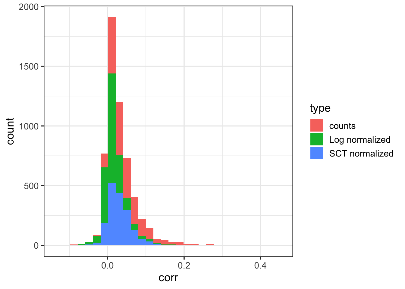
Linear Dimensionality reduction
While we measured around 17000 genes, the “intrinsic” dimensionality of data is smaller - we do not expect all 17000 genes to be orthogonal (“independent” measurements). There will be “modules” of genes that are co-expressed. We want to reduce the dimensioanloty of this dataset to a) enhance the signal to noise ratio and b) visualize this information. A common strategy in this case is to use Principle Component Analysis (PCA) which is a linear dimensionalty reduction method that outputs a smaller (20-50 usually, but upto n-1 PCs in a n dimensional dataset) orthologonal dimensions.
object <- RunPCA(object = object, npcs = 50, verbose = FALSE)Rather than including all the PCs, we want to retain the most informative PCs. The goal here is to avoid adding extra PCs that might reflect other sources of variation (technical) assuming the major source of variation in the dataset is biological.
One way to visualize the “intrinsic dimensionality” of this dataset is to to see how the variance explained by individual PCs varies in the form of an elbow plot:
ElbowPlot(object, ndims = 30)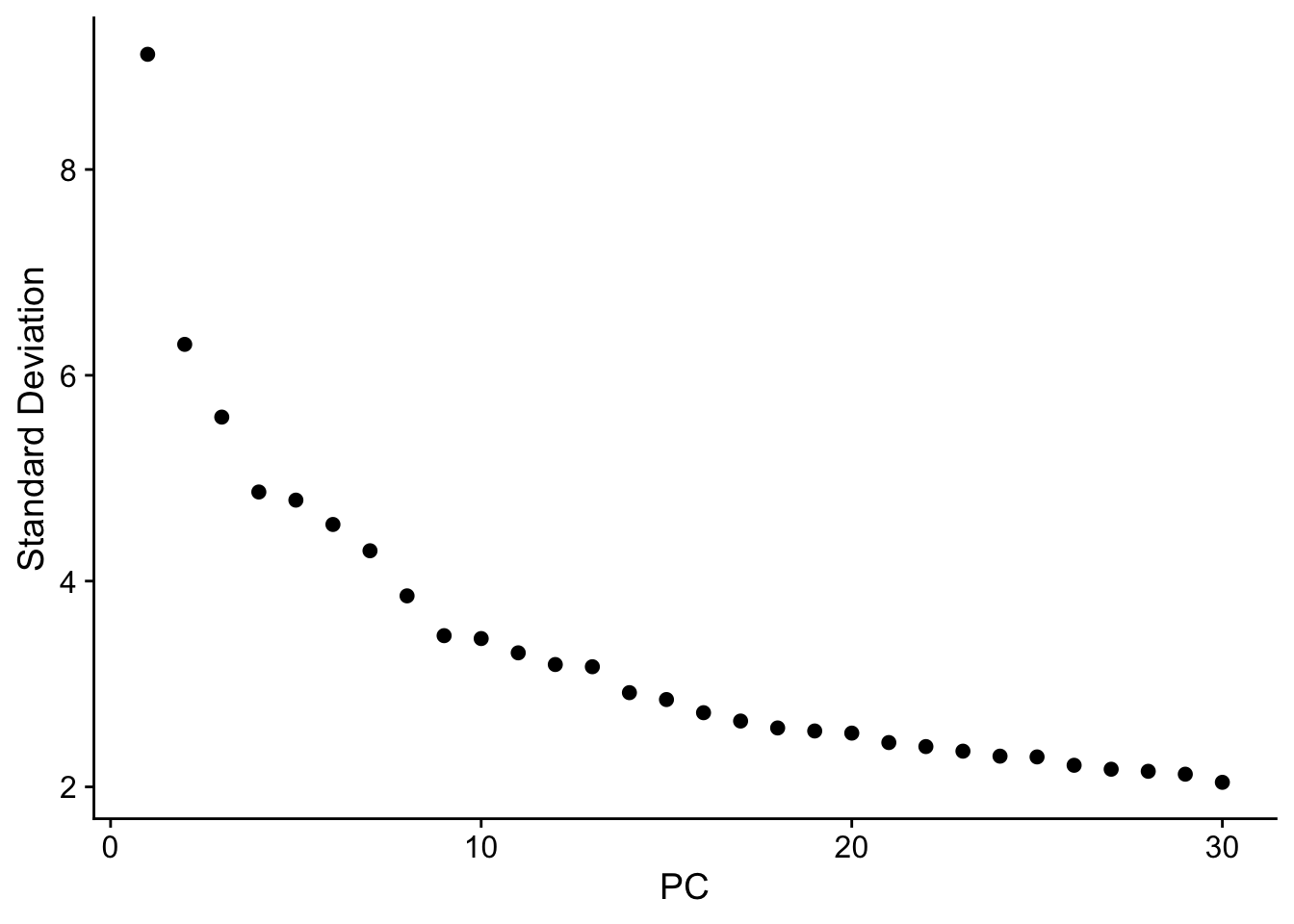
The standard deviation (sequare root of variance) seems to plateau around PC30, so we will retain 30 PCs for downstream visualization and clustering.
Non linear dimensionality reduction
While he previous PCA analysis resulted in 30 dimensions, we want to further reduce the dimension of our dataset to 2 to be able to visualize it. While there are different methods to do this, we will utilize Uniform Manifold Approximation and Projection (UMAP). The goal of UMAP and related dimensionality reduction methods is to find a set of 2-D coordinates for the multidimensional input dataset such that the difference in cell-cell similarities between the low-dimensional and original-dimension dataset is minimized.
object <- RunUMAP(object, reduction = "pca", dims = 1:30)Warning: The default method for RunUMAP has changed from calling Python UMAP via reticulate to the R-native UWOT using the cosine metric
To use Python UMAP via reticulate, set umap.method to 'umap-learn' and metric to 'correlation'
This message will be shown once per session09:52:57 UMAP embedding parameters a = 0.9922 b = 1.11209:52:57 Read 27999 rows and found 30 numeric columns09:52:57 Using Annoy for neighbor search, n_neighbors = 3009:52:57 Building Annoy index with metric = cosine, n_trees = 500% 10 20 30 40 50 60 70 80 90 100%[----|----|----|----|----|----|----|----|----|----|**************************************************|
09:52:59 Writing NN index file to temp file /var/folders/gl/sfjd74gn0wv11h31lr8v2cj40000gn/T//RtmpACrsxU/file177125f977985
09:52:59 Searching Annoy index using 1 thread, search_k = 3000
09:53:03 Annoy recall = 100%
09:53:04 Commencing smooth kNN distance calibration using 1 thread with target n_neighbors = 30
09:53:04 Initializing from normalized Laplacian + noise (using RSpectra)
09:53:05 Commencing optimization for 200 epochs, with 1257072 positive edges
09:53:05 Using rng type: pcg
09:53:13 Optimization finishedDimPlot(object)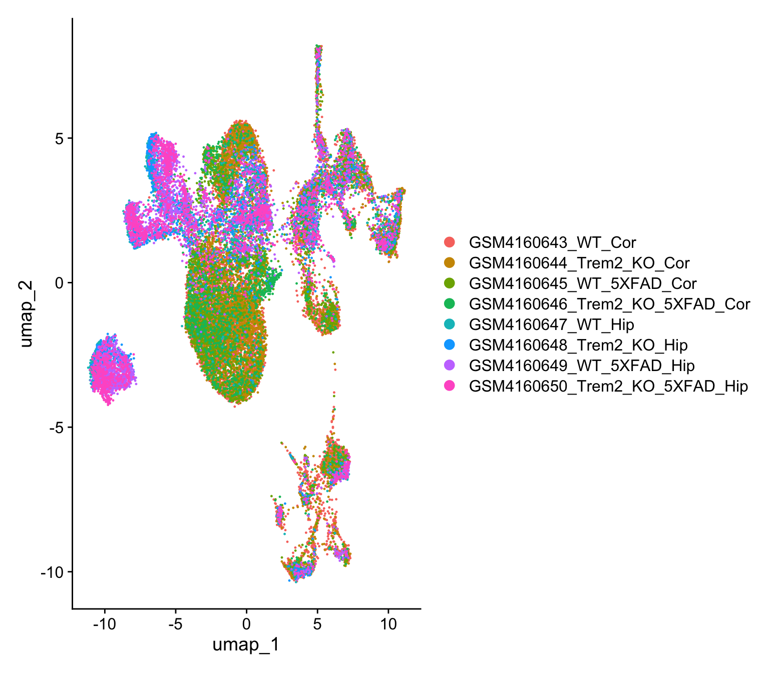
The above plot shows how individual cells are located in a 2D space (defined by the UMAP coordinates). Our dataset is finally ready for a deeper dive in the biology.
Clustering
We can now find “clusters” of cells that likely represent the same celltype. For single-cell data, a popular choice of methods for clustering is graph-based community detection methods that can scale to millions of cells (as opposed to tree-based methods such as hierechial clustering):
# build SNN graph
object <- FindNeighbors(object, reduction = "pca", dims = 1:30)
Computing nearest neighbor graphComputing SNNobject <- FindClusters(object, resolution = 0.3)Modularity Optimizer version 1.3.0 by Ludo Waltman and Nees Jan van Eck
Number of nodes: 27999
Number of edges: 1009506
Running Louvain algorithm...
Maximum modularity in 10 random starts: 0.9347
Number of communities: 17
Elapsed time: 5 secondsDimPlot(object, label = TRUE)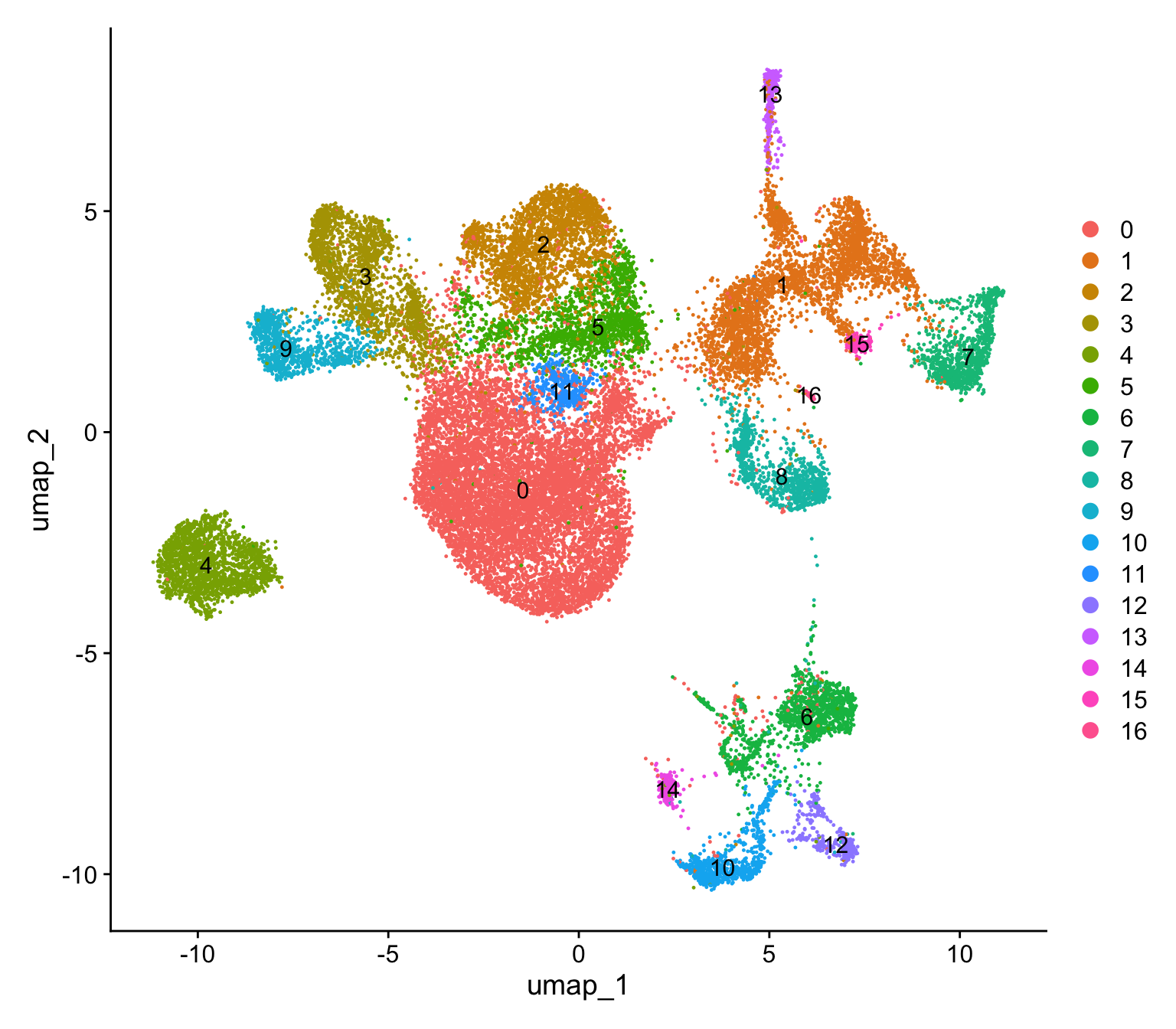
Identifying Microglia cluster
We can visualize some of the marker genes that define the Microglia (See Figure 2 in the associated paper)
FeaturePlot(object, features = c("C1qa", "Fcrls", "Tyrobp", "Csf1r", "Cx3cr1", "P2ry12"))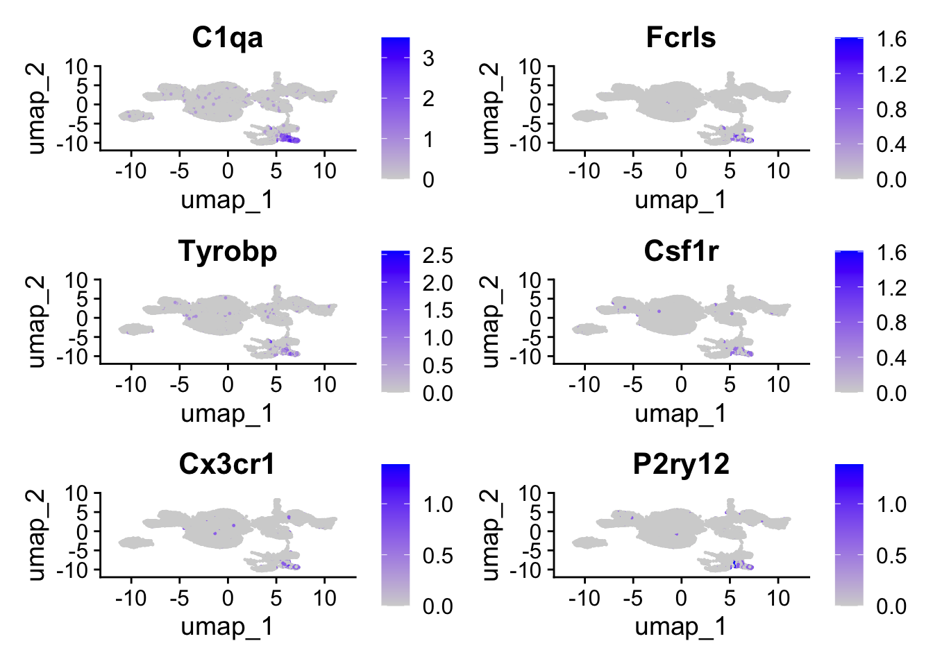
While we can clearly see which cells have highe expression of these genes on the UMAP, it is not clear which “cluster” these cells belong to. You can use VlnPlot to plot the expression pattern of these genes:
VlnPlot(object, features = c("C1qa", "Fcrls", "Tyrobp", "Csf1r", "Cx3cr1", "P2ry12"))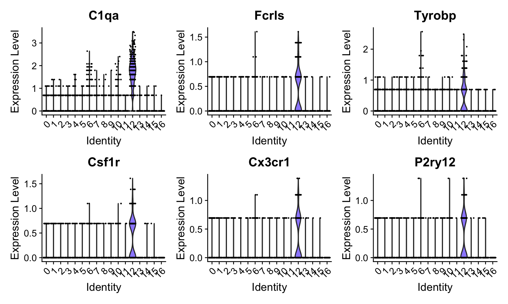
So Cluster 12 is our microglia cluster, we can separate it out to do a deeper analysis
# subset out cluster 12
all.microglia <- subset(object, idents = "12")
Find differentiating markers between the 5XFAD (AD) mouse and the WT mouse
Our next goal is to decipher what genes are differentially expressed in the 5XFAD mouse as compared to the WT mouse (we expect there to be some genes that will be highly expressed in WT and lowly expressed in 5X5AD and vice-versa).
To find differentially expressed (DE) genes, we first set the “identity” of the cells to be the “mouse_model” metadata column and then identify diferentially expressed genes in the 5XFAD mouse as compared to the “WT” mouse using the FindMarkers command:
# Assign the identity to be the mouse model
# among the 'mouse_model` labeled 5XFAD we have both the original 5XFAD (labeled as 'WT' under `genotype` column) and a 'TREM2KO' reflecting the TREM2KO which we remove for this part of the analysis

microglia.notrem2ko <- subset(all.microglia, genotype %in% c("WT"))


Idents(microglia.notrem2ko) <- "mouse_model"

markers.wt_vs_5ad <- FindMarkers(microglia.notrem2ko, ident.1 = "5XFAD", ident.2 = "WT")
markers.wt_vs_5ad$gene <- rownames(markers.wt_vs_5ad)
head(markers.wt_vs_5ad)
p_val avg_log2FC pct.1 pct.2 p_val_adj gene
Cst7 7.936308e-21 5.228819 0.455 0.011 1.345522e-16 Cst7
Thy1 8.935298e-13 2.130032 0.750 0.417 1.514890e-08 Thy1
Ctsd 1.136920e-11 1.388482 0.955 0.911 1.927534e-07 Ctsd
Apoe 8.492906e-10 1.177920 0.932 0.794 1.439887e-05 Apoe
Cd74 4.505810e-09 3.056268 0.261 0.028 7.639151e-05 Cd74
Lyz2 4.938580e-09 1.785782 0.489 0.156 8.372869e-05 Lyz2To visualize these genes we will make use of a “volcano plot” where on the x-axis we will plot the log fold change of each gene and the associated p-value will be plotted on the y-axis. Additinally we will also highlight top 10 DE genes in both directions (positive, i.e. upregulated in 5XFAD and negative, i.e. downregulated in 5XFAD).
library(ggrepel) # load this library to plot gene names

markers.wt_vs_5ad.top10.pos <- markers.wt_vs_5ad %>%
  filter(avg_log2FC>0) %>% filter(p_val_adj<0.05) %>% top_n(n = 10, wt = avg_log2FC)
markers.wt_vs_5ad.top10.neg <- markers.wt_vs_5ad  %>%
   filter(avg_log2FC<0) %>%
  filter(p_val_adj<0.05) %>% top_n(n = 10, wt = abs(avg_log2FC))
markers.wt_vs_5ad.top10 <- rbind(markers.wt_vs_5ad.top10.pos, markers.wt_vs_5ad.top10.neg)

ggplot(markers.wt_vs_5ad, aes(avg_log2FC , -log10(p_val))) +
  geom_point() +
  geom_point(data = markers.wt_vs_5ad.top10, aes(avg_log2FC , -log10(p_val)), color="red" ) +
  geom_text_repel(data = markers.wt_vs_5ad.top10, aes(avg_log2FC, -log10(p_val), label = gene)) + xlab("average log2 Fold Change") + ylab("-log10(Pvalue)")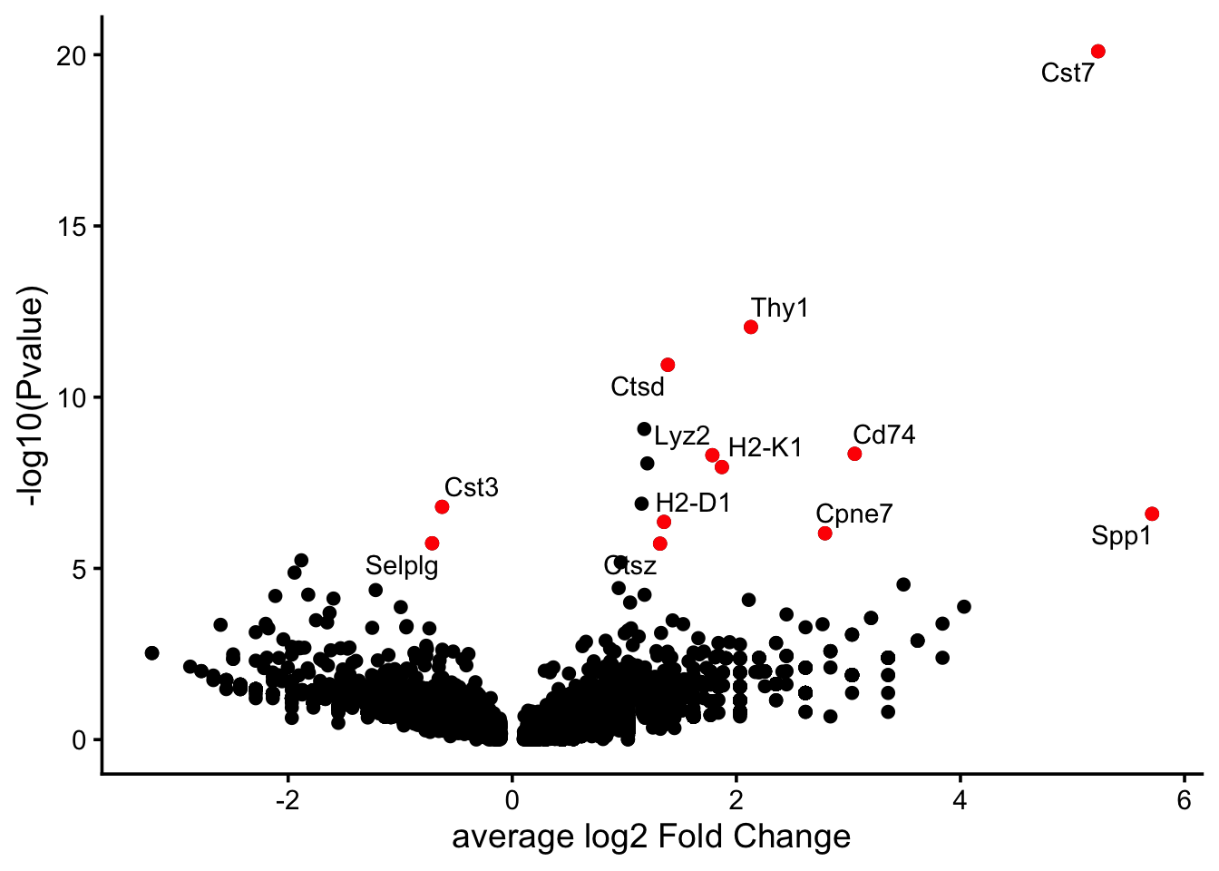
Functional enrichment
On obvious question to ask with the list of DE genes is what function are these carrying? We can perform a gene ontology enrichment using the gene lists to see what functional categories is each of the DE list enriched in.
library(clusterProfiler)clusterProfiler v4.16.0 Learn more at https://yulab-smu.top/contribution-knowledge-mining/
Please cite:
G Yu. Thirteen years of clusterProfiler. The Innovation. 2024,
5(6):100722
Attaching package: 'clusterProfiler'The following object is masked from 'package:purrr':
simplifyThe following object is masked from 'package:stats':
filterlibrary(org.Mm.eg.db) # install using BiocManager::install("org.Mm.eg.db")Loading required package: AnnotationDbiLoading required package: stats4Loading required package: BiocGenericsLoading required package: generics
Attaching package: 'generics'The following object is masked from 'package:lubridate':
as.difftimeThe following object is masked from 'package:dplyr':
explainThe following objects are masked from 'package:base':
as.difftime, as.factor, as.ordered, intersect, is.element, setdiff,
setequal, union
Attaching package: 'BiocGenerics'The following object is masked from 'package:dplyr':
combineThe following objects are masked from 'package:stats':
IQR, mad, sd, var, xtabsThe following objects are masked from 'package:base':
anyDuplicated, aperm, append, as.data.frame, basename, cbind,
colnames, dirname, do.call, duplicated, eval, evalq, Filter, Find,
get, grep, grepl, is.unsorted, lapply, Map, mapply, match, mget,
order, paste, pmax, pmax.int, pmin, pmin.int, Position, rank,
rbind, Reduce, rownames, sapply, saveRDS, table, tapply, unique,
unsplit, which.max, which.minLoading required package: BiobaseWelcome to Bioconductor
Vignettes contain introductory material; view with
'browseVignettes()'. To cite Bioconductor, see
'citation("Biobase")', and for packages 'citation("pkgname")'.Loading required package: IRangesLoading required package: S4Vectors
Attaching package: 'S4Vectors'The following object is masked from 'package:clusterProfiler':
renameThe following objects are masked from 'package:lubridate':
second, second<-The following objects are masked from 'package:dplyr':
first, renameThe following object is masked from 'package:tidyr':
expandThe following object is masked from 'package:utils':
findMatchesThe following objects are masked from 'package:base':
expand.grid, I, unname
Attaching package: 'IRanges'The following object is masked from 'package:clusterProfiler':
sliceThe following object is masked from 'package:lubridate':
%within%The following objects are masked from 'package:dplyr':
collapse, desc, sliceThe following object is masked from 'package:purrr':
reduceThe following object is masked from 'package:sp':
%over%
Attaching package: 'AnnotationDbi'The following object is masked from 'package:clusterProfiler':
selectThe following object is masked from 'package:dplyr':
selectuniverse.genes <- rownames(counts)
DoEnrichment <- function(genes, universe.genes) {
enrich <- enrichGO(gene = genes,
universe = universe.genes,
OrgDb = org.Mm.eg.db,
keyType = "SYMBOL",
ont = "BP",
pvalueCutoff = 0.05,
qvalueCutoff = 0.05,
readable = TRUE)
return(enrich)
}
de.pos <- markers.wt_vs_5ad %>%
filter(avg_log2FC>0) %>% filter(p_val_adj<0.1) %>% pull (gene)
de.neg <- markers.wt_vs_5ad %>%
filter(avg_log2FC<0) %>% filter(p_val_adj<0.1) %>% pull (gene)
enrichment.pos <- DoEnrichment(genes = de.pos, universe.genes = universe.genes)
enrichment.neg <- DoEnrichment(genes = de.neg, universe.genes = universe.genes)barplot(enrichment.pos)+ ggtitle("Enrichment of 5XFAD upregulated genes")Warning in fortify(object, showCategory = showCategory, by = x, ...): Arguments in `...` must be used.
✖ Problematic argument:
• by = x
ℹ Did you misspell an argument name?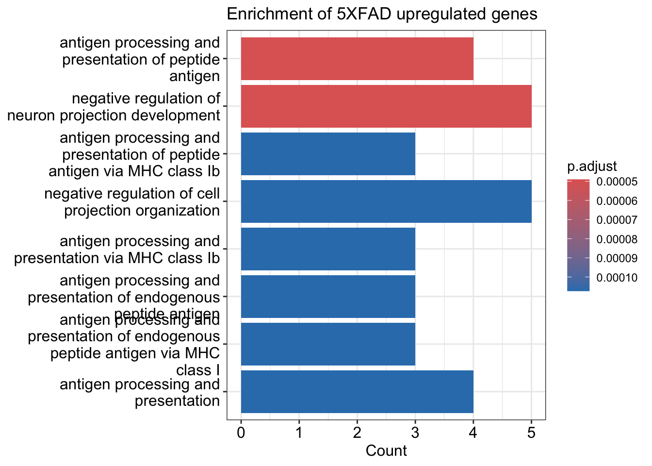
barplot(enrichment.neg, showTerms = 7) + ggtitle("Enrichment of 5XFAD downregulated genes")Warning in fortify(object, showCategory = showCategory, by = x, ...): Arguments in `...` must be used.
✖ Problematic arguments:
• by = x
• showTerms = 7
ℹ Did you misspell an argument name?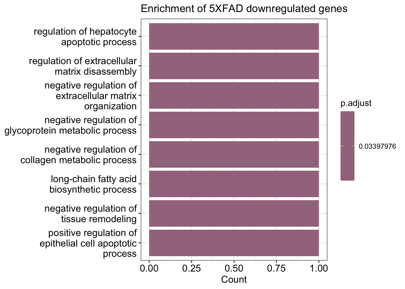
We should compare your results with the following claim in the paper:
DAM genes, including Cst7, Csf1, Apoe, Trem2, Lpl, Lilrb4a, H2-d1 (an MHC-I gene), Cd74 (an MHC-II-related gene) and various cathepsin genes were notably upregulated in 5XFAD compared with WT mice. Homeostatic genes, such as P2ry12, Selplg, Tmem119 and Cx3cr1, were downregulated. These results were highly concordant between the 7-month- and 15-month-old datasets (Fig. 2d) and with previously published single-cell RNAseq data of sorted microglia.
List of genes upregulated in 5XFAD:
de.pos [1] "Cst7" "Thy1" "Ctsd" "Apoe" "Cd74" "Lyz2" "B2m" "H2-K1" "Ctsb"
[10] "Spp1" "H2-D1" "Cpne7" "Ctsz" List of genes downregulated in 5XFAD:
de.neg[1] "Cst3" "Selplg" "Plp1" Exercise
Identify what genes are differentially expressed in 5XFAD mouse as compared to the WT mouse.
Reveal solution
The mouse_model column stores the information about it being a WT or an AD (5XFAD) mouse. In this study the authors were also interested in asking what changes happen to the microglial gene program if TREM2 is knocked out (given the prior knowledge about microglial transcriptional response dependence on TREM2). In the above analysis we removed cells that were not labeled as “WT” under their “genotype” column. Here we will subset a different set of cells which are all “5XFAD” but can have different genotype (“WT” or “TREM2KO”)
microglia.5xfad <- subset(all.microglia, mouse_model %in% c("5XFAD"))

# now we set the identities to the genotype
Idents(microglia.5xfad) <- "genotype"
markers.5ad_vs_trem2ko <- FindMarkers(microglia.5xfad, ident.1 = "WT", ident.2 = "Trem2KO")
markers.5ad_vs_trem2ko$gene <- rownames(markers.5ad_vs_trem2ko)
head(markers.5ad_vs_trem2ko)
p_val avg_log2FC pct.1 pct.2 p_val_adj gene
Trem2 9.850060e-10 4.358352 0.920 0.105 1.669979e-05 Trem2
Cfap20 1.371005e-04 -3.211504 0.023 0.263 1.000000e+00 Cfap20
Ubqln2 1.778727e-04 -4.211504 0.000 0.158 1.000000e+00 Ubqln2
Col16a1 1.778727e-04 -4.211504 0.000 0.158 1.000000e+00 Col16a1
Cep135 1.778727e-04 -4.211504 0.000 0.158 1.000000e+00 Cep135
Ddx25 1.778727e-04 -4.211504 0.000 0.158 1.000000e+00 Ddx25markers.5ad_vs_trem2ko.top10.pos <- markers.5ad_vs_trem2ko %>%
filter(avg_log2FC>0) %>% filter(p_val_adj<0.05) %>% top_n(n = 10, wt = avg_log2FC)
markers.5ad_vs_trem2ko.top10.neg <- markers.5ad_vs_trem2ko %>%
filter(avg_log2FC<0) %>%
filter(p_val_adj<0.05) %>% top_n(n = 10, wt = abs(avg_log2FC))
markers.5ad_vs_trem2ko.top10 <- rbind(markers.5ad_vs_trem2ko.top10.pos, markers.5ad_vs_trem2ko.top10.neg)
ggplot(markers.5ad_vs_trem2ko, aes(avg_log2FC , -log10(p_val))) +
geom_point() +
geom_point(data = markers.5ad_vs_trem2ko.top10, aes(avg_log2FC , -log10(p_val)), color="red" ) +
geom_text_repel(data = markers.5ad_vs_trem2ko.top10, aes(avg_log2FC, -log10(p_val), label = gene)) + xlab("average log2 Fold Change") + ylab("-log10(Pvalue)")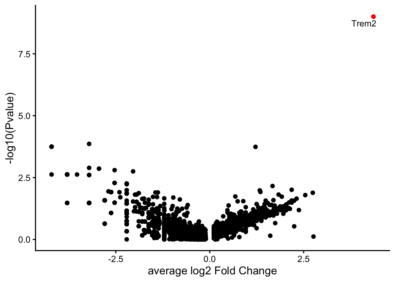
Session Info
sessionInfo()R version 4.5.1 (2025-06-13)
Platform: aarch64-apple-darwin20
Running under: macOS Tahoe 26.0.1
Matrix products: default
BLAS: /Library/Frameworks/R.framework/Versions/4.5-arm64/Resources/lib/libRblas.0.dylib
LAPACK: /Library/Frameworks/R.framework/Versions/4.5-arm64/Resources/lib/libRlapack.dylib; LAPACK version 3.12.1
locale:
[1] en_US.UTF-8/en_US.UTF-8/en_US.UTF-8/C/en_US.UTF-8/en_US.UTF-8
time zone: Asia/Kolkata
tzcode source: internal
attached base packages:
[1] stats4 stats graphics grDevices utils datasets methods
[8] base
other attached packages:
[1] org.Mm.eg.db_3.21.0 AnnotationDbi_1.70.0 IRanges_2.42.0
[4] S4Vectors_0.46.0 Biobase_2.68.0 BiocGenerics_0.54.1
[7] generics_0.1.4 clusterProfiler_4.16.0 ggrepel_0.9.6
[10] future_1.67.0 lubridate_1.9.4 forcats_1.0.1
[13] stringr_1.5.2 dplyr_1.1.4 purrr_1.1.0
[16] readr_2.1.5 tidyr_1.3.1 tibble_3.3.0
[19] ggplot2_4.0.0 tidyverse_2.0.0 Seurat_5.3.0
[22] SeuratObject_5.2.0 sp_2.2-0
loaded via a namespace (and not attached):
[1] RcppAnnoy_0.0.22 splines_4.5.1
[3] later_1.4.4 ggplotify_0.1.3
[5] R.oo_1.27.1 polyclip_1.10-7
[7] fastDummies_1.7.5 lifecycle_1.0.4
[9] rprojroot_2.1.1 globals_0.18.0
[11] lattice_0.22-7 MASS_7.3-65
[13] magrittr_2.0.4 limma_3.64.3
[15] plotly_4.11.0 rmarkdown_2.30
[17] yaml_2.3.10 ggtangle_0.0.7
[19] httpuv_1.6.16 glmGamPoi_1.20.0
[21] sctransform_0.4.2 spam_2.11-1
[23] spatstat.sparse_3.1-0 reticulate_1.43.0
[25] cowplot_1.2.0 pbapply_1.7-4
[27] DBI_1.2.3 RColorBrewer_1.1-3
[29] abind_1.4-8 Rtsne_0.17
[31] GenomicRanges_1.60.0 R.utils_2.13.0
[33] presto_1.0.0 yulab.utils_0.2.1
[35] rappdirs_0.3.3 GenomeInfoDbData_1.2.14
[37] enrichplot_1.28.4 irlba_2.3.5.1
[39] listenv_0.9.1 spatstat.utils_3.2-0
[41] tidytree_0.4.6 goftest_1.2-3
[43] RSpectra_0.16-2 spatstat.random_3.4-2
[45] fitdistrplus_1.2-4 parallelly_1.45.1
[47] DelayedMatrixStats_1.30.0 codetools_0.2-20
[49] DelayedArray_0.34.1 DOSE_4.2.0
[51] tidyselect_1.2.1 aplot_0.2.9
[53] UCSC.utils_1.4.0 farver_2.1.2
[55] matrixStats_1.5.0 spatstat.explore_3.5-3
[57] jsonlite_2.0.0 progressr_0.16.0
[59] ggridges_0.5.7 survival_3.8-3
[61] tools_4.5.1 treeio_1.32.0
[63] ica_1.0-3 Rcpp_1.1.0
[65] glue_1.8.0 gridExtra_2.3
[67] SparseArray_1.8.1 xfun_0.53
[69] here_1.0.2 qvalue_2.40.0
[71] MatrixGenerics_1.20.0 GenomeInfoDb_1.44.3
[73] withr_3.0.2 fastmap_1.2.0
[75] digest_0.6.37 gridGraphics_0.5-1
[77] timechange_0.3.0 R6_2.6.1
[79] mime_0.13 colorspace_2.1-2
[81] GO.db_3.21.0 scattermore_1.2
[83] tensor_1.5.1 dichromat_2.0-0.1
[85] spatstat.data_3.1-8 RSQLite_2.4.3
[87] R.methodsS3_1.8.2 data.table_1.17.8
[89] httr_1.4.7 htmlwidgets_1.6.4
[91] S4Arrays_1.8.1 uwot_0.2.3
[93] pkgconfig_2.0.3 gtable_0.3.6
[95] blob_1.2.4 lmtest_0.9-40
[97] S7_0.2.0 XVector_0.48.0
[99] htmltools_0.5.8.1 fgsea_1.34.2
[101] dotCall64_1.2 scales_1.4.0
[103] png_0.1-8 spatstat.univar_3.1-4
[105] ggfun_0.2.0 knitr_1.50
[107] rstudioapi_0.17.1 tzdb_0.5.0
[109] reshape2_1.4.4 nlme_3.1-168
[111] cachem_1.1.0 zoo_1.8-14
[113] KernSmooth_2.23-26 parallel_4.5.1
[115] miniUI_0.1.2 vipor_0.4.7
[117] ggrastr_1.0.2 pillar_1.11.1
[119] grid_4.5.1 vctrs_0.6.5
[121] RANN_2.6.2 promises_1.3.3
[123] beachmat_2.24.0 xtable_1.8-4
[125] cluster_2.1.8.1 beeswarm_0.4.0
[127] evaluate_1.0.5 cli_3.6.5
[129] compiler_4.5.1 rlang_1.1.6
[131] crayon_1.5.3 future.apply_1.20.0
[133] labeling_0.4.3 fs_1.6.6
[135] plyr_1.8.9 ggbeeswarm_0.7.2
[137] stringi_1.8.7 BiocParallel_1.42.2
[139] viridisLite_0.4.2 deldir_2.0-4
[141] Biostrings_2.76.0 lazyeval_0.2.2
[143] spatstat.geom_3.6-0 GOSemSim_2.34.0
[145] Matrix_1.7-4 RcppHNSW_0.6.0
[147] hms_1.1.3 patchwork_1.3.2
[149] sparseMatrixStats_1.20.0 bit64_4.6.0-1
[151] KEGGREST_1.48.1 statmod_1.5.1
[153] shiny_1.11.1 SummarizedExperiment_1.38.1
[155] ROCR_1.0-11 memoise_2.0.1
[157] igraph_2.2.0 ggtree_3.16.3
[159] fastmatch_1.1-6 bit_4.6.0
[161] gson_0.1.0 ape_5.8-1