---
title: "Regularized regression"
---
# Introduction
This notebook demonstrates five regularized regression methods using the classic **Prostate Cancer Dataset** (Stamey et al., 1989).
## Dataset
The prostate cancer dataset contains measurements from **97 men** with prostate cancer who were about to receive radical prostatectomy. The goal is to predict log(PSA) levels based on clinical measurements.
```{r setup}
#| label: setup
#| code-summary: "Load packages"
required_packages <- c(
  "glmnet", "pls", "MASS", "patchwork",
  "reshape2", "tidyr", "dplyr", "tidyverse"
)

new_packages <- required_packages[!(required_packages %in% installed.packages()[, "Package"])]
if (length(new_packages)) install.packages(new_packages)

library(glmnet) # For Ridge, Lasso, Elastic Net
library(pls) # For PLS and PCR
library(MASS) # For additional statistical functions
library(ggplot2) # For visualizations
library(patchwork) # For arranging multiple plots
library(reshape2) # For data manipulation
library(tidyr) # For data tidying
library(dplyr) # For data manipulation
theme_set(theme_minimal(base_size = 12))
```
```{r load-data}
#| label: load-data
#| code-summary: "Load prostate cancer data"
prostate_url <- "https://hastie.su.domains/ElemStatLearn/datasets/prostate.data"
prostate <- read.table(prostate_url, header = TRUE, row.names = 1)
```
## Data overview
```{r data-overview}
#| label: data-overview
#| code-summary: "View data structure"
head(prostate)
summary(prostate)
```
::: {.callout-tip}
## Variable Descriptions
- `lcavol`: log(cancer volume)
- `lweight`: log(prostate weight)
- `age`: patient age in years
- `lbph`: log(benign prostatic hyperplasia amount)
- `svi`: seminal vesicle invasion (0/1)
- `lcp`: log(capsular penetration)
- `gleason`: Gleason score (6-9)
- `pgg45`: percentage Gleason scores 4 or 5
- `lpsa`: log(PSA) - **outcome variable**
- `train`: training set indicator
:::
## Prepare data
```{r data-prep}
#| label: data-prep
#| code-summary: "Prepare train/test splits"
train_data <- prostate[prostate$train == TRUE, ]
test_data <- prostate[prostate$train == FALSE, ]

train_data <- train_data[, -10]
test_data <- test_data[, -10]

# All predictors
x_train <- as.matrix(train_data[, -9])
y_train <- train_data$lpsa

x_test <- as.matrix(test_data[, -9])
y_test <- test_data$lpsa

# Standardize predictors --> Imp
x_train_scaled <- scale(x_train)
x_test_scaled <- scale(x_test,
  center = attr(x_train_scaled, "scaled:center"),
  scale = attr(x_train_scaled, "scaled:scale")
)
```
```{r}
cat("Training set size:", nrow(train_data), "\n")
cat("Test set size:", nrow(test_data), "\n")
cat("Number of predictors:", ncol(x_train), "\n")
```
## EDA
### Correlations across features
```{r correlation-plot}
#| label: fig-correlation
#| fig-cap: "Correlation matrix showing relationships among predictors."
#| code-summary: "Create correlation heatmap"
cor_matrix <- cor(x_train)

get_upper_tri <- function(cormat) {
  cormat[lower.tri(cormat)] <- NA
  return(cormat)
}
upper_tri <- get_upper_tri(cor_matrix)
cor_melted <- melt(upper_tri, na.rm = TRUE)

p_corr <- ggplot(cor_melted, aes(Var1, Var2, fill = value)) +
  geom_tile(color = "white") +
  geom_text(aes(label = sprintf("%.2f", value)), size = 3) +
  scale_fill_gradient2(
    low = "blue", high = "red", mid = "white",
    midpoint = 0, limit = c(-1, 1),
    name = "Correlation"
  ) +
  theme_minimal(base_size = 11) +
  theme(
    axis.text.x = element_text(angle = 45, hjust = 1),
    axis.title.x = element_blank(),
    axis.title.y = element_blank()
  ) +
  labs(title = "Correlation Matrix of Prostate Cancer Predictors") +
  coord_fixed()

p_corr
```
Note the high correlation between lcavol and lcp (0.69) --> multicollinearity!
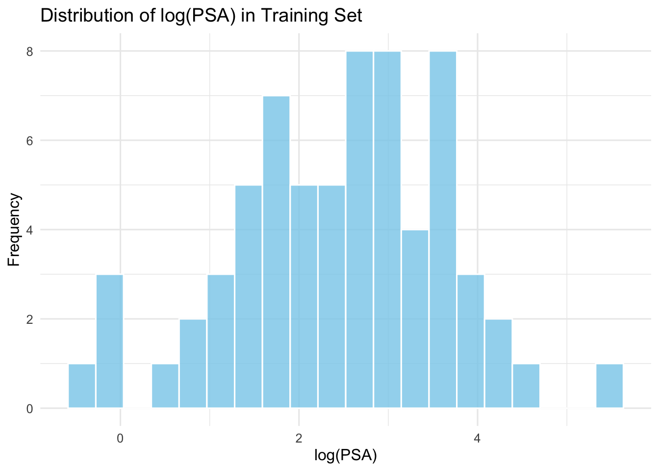
### Response variable description
```{r response-dist}
#| label: fig-response
#| fig-cap: "Distribution of log(PSA) in the training set."
#| code-summary: "Plot response variable"
p_dist <- ggplot(data.frame(lpsa = y_train), aes(x = lpsa)) +
  geom_histogram(bins = 20, fill = "skyblue", color = "white", alpha = 0.8) +
  labs(
    title = "Distribution of log(PSA) in Training Set",
    x = "log(PSA)", y = "Frequency"
  ) +
  theme_minimal(base_size = 12)

p_dist
```
::: {.callout-important}
The distribution is approximately normal, which is suitable for regression analysis. However, the correlation matrix reveals multicollinearity among predictors, particularly between:
- `lcavol` and `lcp` (r = 0.69)
- `lcavol` and `svi` (r = 0.59)
This makes regularization methods particularly valuable for this dataset.
:::
# OLS (Baseline) {#sec-ols}
Before applying regularization, let's fit a standard multiple linear regression model (OLS) as our baseline for comparison.
```{r ols-fit}
#| label: ols-fit
#| code-summary: "Fit ordinary least squares regression"
ols_model <- lm(lpsa ~ ., data = train_data)

ols_pred_train <- predict(ols_model, newdata = train_data)
ols_pred_test <- predict(ols_model, newdata = test_data)

ols_train_mse <- mean((y_train - ols_pred_train)^2)
ols_test_mse <- mean((y_test - ols_pred_test)^2)
ols_train_rmse <- sqrt(ols_train_mse)
ols_test_rmse <- sqrt(ols_test_mse)
ols_train_r2 <- summary(ols_model)$r.squared
ols_test_r2 <- 1 - sum((y_test - ols_pred_test)^2) / sum((y_test - mean(y_test))^2)
```
```{r}
cat("OLS Train MSE:", round(ols_train_mse, 4), "\n")
cat("OLS Test MSE:", round(ols_test_mse, 4), "\n")
cat("OLS Train RMSE:", round(ols_train_rmse, 4), "\n")
cat("OLS Test RMSE:", round(ols_test_rmse, 4), "\n")
cat("OLS Train R²:", round(ols_train_r2, 4), "\n")
cat("OLS Test R²:", round(ols_test_r2, 4), "\n")
print(summary(ols_model))
```
::: {.callout-note}
## OLS - the baseline
The ordinary least squares model provides an unregularized baseline. With 8 predictors and 67 training observations, OLS may overfit, especially given the multicollinearity we observed.
:::
# Ridge regression {#sec-ridge}
Ridge regression applies an L2 penalty to the coefficients, shrinking them toward zero but **never exactly to zero**. This is particularly effective for handling multicollinearity.
$$\min_{\beta} \sum_{i=1}^{n} (y_i - \beta_0 - \sum_{j=1}^{p} x_{ij}\beta_j)^2 + \lambda \sum_{j=1}^{p} \beta_j^2$$
```{r ridge-fit}
#| label: ridge-fit
#| code-summary: "Fit ridge regression"
set.seed(123)
# see: https://glmnet.stanford.edu/articles/glmnet.html
ridge_cv <- cv.glmnet(x_train_scaled, y_train, alpha = 0, nfolds = 10)

# optimal lambda
cat("Optimal lambda (Ridge):", ridge_cv$lambda.min, "\n")
# ridge fit
ridge_model <- glmnet(x_train_scaled, y_train,
  alpha = 0,
  lambda = ridge_cv$lambda.min
)

# Predict
ridge_pred_train <- predict(ridge_model, newx = x_train_scaled)
ridge_pred_test <- predict(ridge_model, newx = x_test_scaled)

# Performance metrics
ridge_train_mse <- mean((y_train - ridge_pred_train)^2)
ridge_test_mse <- mean((y_test - ridge_pred_test)^2)
ridge_train_rmse <- sqrt(ridge_train_mse)
ridge_test_rmse <- sqrt(ridge_test_mse)
ridge_train_r2 <- 1 - sum((y_train - ridge_pred_train)^2) / sum((y_train - mean(y_train))^2)
ridge_test_r2 <- 1 - sum((y_test - ridge_pred_test)^2) / sum((y_test - mean(y_test))^2)
```
```{r}
cat("Ridge Train MSE:", round(ridge_train_mse, 4), "\n")
cat("Ridge Test MSE:", round(ridge_test_mse, 4), "\n")
cat("Ridge Train RMSE:", round(ridge_train_rmse, 4), "\n")
cat("Ridge Test RMSE:", round(ridge_test_rmse, 4), "\n")
cat("Ridge Train R²:", round(ridge_train_r2, 4), "\n")
cat("Ridge Test R²:", round(ridge_test_r2, 4), "\n")
```
## Ridge Visualizations
```{r ridge-viz}
#| label: fig-ridge
#| fig-cap: "Ridge regression cross-validation and coefficient paths. Left: CV error as a function of lambda. Right: How coefficients shrink as regularization increases."
#| fig-width: 14
#| fig-height: 6
#| code-summary: "Create ridge visualizations"
# Lambda selection
ridge_cv_df <- data.frame(
  lambda = ridge_cv$lambda,
  cvm = ridge_cv$cvm,
  cvlo = ridge_cv$cvlo,
  cvup = ridge_cv$cvup
)

p_ridge_cv <- ggplot(ridge_cv_df, aes(x = log(lambda), y = cvm)) +
  geom_point(color = "red", size = 2) +
  geom_errorbar(aes(ymin = cvlo, ymax = cvup), width = 0.1, alpha = 0.5) +
  geom_vline(xintercept = log(ridge_cv$lambda.min), linetype = "dashed", color = "blue") +
  geom_vline(xintercept = log(ridge_cv$lambda.1se), linetype = "dashed", color = "darkgreen") +
  labs(
    title = "Ridge regression: Cross-validation",
    x = "log(Lambda)",
    y = "Mean-squared error"
  ) +
  annotate("text",
    x = log(ridge_cv$lambda.min), y = max(ridge_cv_df$cvm),
    label = "lambda.min", hjust = -0.1, color = "blue"
  ) +
  theme_minimal(base_size = 12)
```
```{r}
# Coefficient paths
ridge_full <- glmnet(x_train_scaled, y_train, alpha = 0)
ridge_coef_df <- as.data.frame(as.matrix(t(ridge_full$beta)))
ridge_coef_df$lambda <- ridge_full$lambda
ridge_coef_long <- pivot_longer(ridge_coef_df,
  cols = -lambda,
  names_to = "variable", values_to = "coefficient"
)

p_ridge_path <- ggplot(ridge_coef_long, aes(x = log(lambda), y = coefficient, color = variable)) +
  geom_line(linewidth = 1) +
  geom_vline(xintercept = log(ridge_cv$lambda.min), linetype = "dashed", color = "red") +
  labs(
    title = "Ridge regression: coefficient paths",
    x = "log(Lambda)",
    y = "Coefficient value",
    color = "Variable"
  ) +
  theme_minimal(base_size = 12) +
  theme(legend.position = "right")

p_ridge_cv + p_ridge_path
```
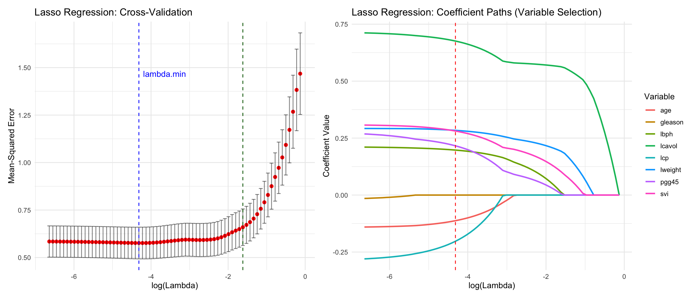
# Lasso regression {#sec-lasso}
Lasso (Least absolute shrinkage and selection operator) applies an L1 penalty, which can **shrink coefficients exactly to zero**, performing automatic variable selection. See [this notebook](ridge_vs_lasso.qmd) for details.
$$\min_{\beta} \sum_{i=1}^{n} (y_i - \beta_0 - \sum_{j=1}^{p} x_{ij}\beta_j)^2 + \lambda \sum_{j=1}^{p} |\beta_j|$$
```{r lasso-fit}
#| label: lasso-fit
#| code-summary: "Fit Lasso"
# fit lasso
set.seed(32)
# see: https://glmnet.stanford.edu/articles/glmnet.html
lasso_cv <- cv.glmnet(x_train_scaled, y_train, alpha = 1, nfolds = 10)


cat("Optimal lambda (Lasso):", lasso_cv$lambda.min, "\n")
lasso_model <- glmnet(x_train_scaled, y_train,
  alpha = 1,
  lambda = lasso_cv$lambda.min
)


lasso_pred_train <- predict(lasso_model, newx = x_train_scaled)
lasso_pred_test <- predict(lasso_model, newx = x_test_scaled)


lasso_train_mse <- mean((y_train - lasso_pred_train)^2)
lasso_test_mse <- mean((y_test - lasso_pred_test)^2)
lasso_train_rmse <- sqrt(lasso_train_mse)
lasso_test_rmse <- sqrt(lasso_test_mse)
lasso_train_r2 <- 1 - sum((y_train - lasso_pred_train)^2) / sum((y_train - mean(y_train))^2)
lasso_test_r2 <- 1 - sum((y_test - lasso_pred_test)^2) / sum((y_test - mean(y_test))^2)
```
```{r}
cat("Lasso Train MSE:", round(lasso_train_mse, 4), "\n")
cat("Lasso Test MSE:", round(lasso_test_mse, 4), "\n")
cat("Lasso Train RMSE:", round(lasso_train_rmse, 4), "\n")
cat("Lasso Test RMSE:", round(lasso_test_rmse, 4), "\n")
cat("Lasso Train R²:", round(lasso_train_r2, 4), "\n")
cat("Lasso Test R²:", round(lasso_test_r2, 4), "\n")
```
```{r}
# Selected variables
lasso_coefs <- coef(lasso_model)
selected_vars <- rownames(lasso_coefs)[lasso_coefs[, 1] != 0]
cat("\nSelected variables by Lasso:", paste(selected_vars[-1], collapse = ", "), "\n")
```
## Lasso - visualise
```{r lasso-viz}
#| label: fig-lasso
#| fig-cap: "Lasso regression cross-validation and coefficient paths. Note how some coefficients are driven exactly to zero, performing automatic variable selection."
#| fig-width: 14
#| fig-height: 6
#| code-summary: "Create Lasso visualizations"
# Lambda selection
lasso_cv_df <- data.frame(
  lambda = lasso_cv$lambda,
  cvm = lasso_cv$cvm,
  cvlo = lasso_cv$cvlo,
  cvup = lasso_cv$cvup
)

p_lasso_cv <- ggplot(lasso_cv_df, aes(x = log(lambda), y = cvm)) +
  geom_point(color = "red", size = 2) +
  geom_errorbar(aes(ymin = cvlo, ymax = cvup), width = 0.1, alpha = 0.5) +
  geom_vline(xintercept = log(lasso_cv$lambda.min), linetype = "dashed", color = "blue") +
  geom_vline(xintercept = log(lasso_cv$lambda.1se), linetype = "dashed", color = "darkgreen") +
  labs(
    title = "Lasso Regression: Cross-Validation",
    x = "log(Lambda)",
    y = "Mean-Squared Error"
  ) +
  annotate("text",
    x = log(lasso_cv$lambda.min), y = max(lasso_cv_df$cvm),
    label = "lambda.min", hjust = -0.1, color = "blue"
  ) +
  theme_minimal(base_size = 12)

# Coefficient paths (shows variable selection)
lasso_full <- glmnet(x_train_scaled, y_train, alpha = 1)
lasso_coef_df <- as.data.frame(as.matrix(t(lasso_full$beta)))
lasso_coef_df$lambda <- lasso_full$lambda
lasso_coef_long <- pivot_longer(lasso_coef_df,
  cols = -lambda,
  names_to = "variable", values_to = "coefficient"
)

p_lasso_path <- ggplot(lasso_coef_long, aes(x = log(lambda), y = coefficient, color = variable)) +
  geom_line(linewidth = 1) +
  geom_vline(xintercept = log(lasso_cv$lambda.min), linetype = "dashed", color = "red") +
  labs(
    title = "Lasso Regression: Coefficient Paths (Variable Selection)",
    x = "log(Lambda)",
    y = "Coefficient Value",
    color = "Variable"
  ) +
  theme_minimal(base_size = 12) +
  theme(legend.position = "right")

p_lasso_cv + p_lasso_path
```
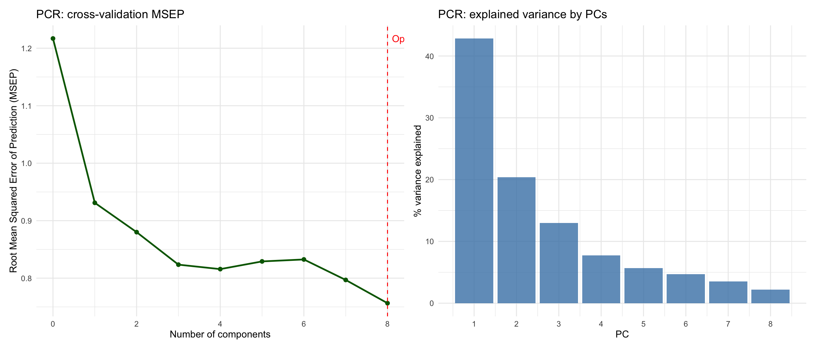
# Principal Component Regression (PCR) {#sec-pcr}
PCR performs **unsupervised dimension reduction** by finding components that maximize variance in the predictors (ignoring the response).
```{r pcr-fit}
#| label: pcr-fit
#| code-summary: "Fit PCR"
train_df <- data.frame(x_train_scaled, lpsa = y_train)
test_df <- data.frame(x_test_scaled, lpsa = y_test)

cat("=== PRINCIPAL COMPONENT REGRESSION ===\n")
# Fit PCR with cross-validation
set.seed(123)
pcr_model <- pcr(lpsa ~ ., data = train_df, validation = "CV", segments = 10)

# Determine optimal number of components
pcr_cv_mse <- RMSEP(pcr_model, estimate = "CV")
optimal_ncomp_pcr <- which.min(pcr_cv_mse$val[1, , ]) - 1
cat("Optimal number of components (PCR):", optimal_ncomp_pcr, "\n")
# Predictions
pcr_pred_train <- predict(pcr_model, newdata = train_df, ncomp = optimal_ncomp_pcr)
pcr_pred_test <- predict(pcr_model, newdata = test_df, ncomp = optimal_ncomp_pcr)

# Performance metrics
pcr_train_mse <- mean((y_train - pcr_pred_train)^2)
pcr_test_mse <- mean((y_test - pcr_pred_test)^2)
pcr_train_rmse <- sqrt(pcr_train_mse)
pcr_test_rmse <- sqrt(pcr_test_mse)
pcr_train_r2 <- 1 - sum((y_train - pcr_pred_train)^2) / sum((y_train - mean(y_train))^2)
pcr_test_r2 <- 1 - sum((y_test - pcr_pred_test)^2) / sum((y_test - mean(y_test))^2)
```
```{r}
cat("PCR Train MSE:", round(pcr_train_mse, 4), "\n")
cat("PCR Test MSE:", round(pcr_test_mse, 4), "\n")
cat("PCR Train RMSE:", round(pcr_train_rmse, 4), "\n")
cat("PCR Test RMSE:", round(pcr_test_rmse, 4), "\n")
cat("PCR Train R²:", round(pcr_train_r2, 4), "\n")
cat("PCR Test R²:", round(pcr_test_r2, 4), "\n")
```
## PCR visualisation
```{r pcr-viz}
#| label: fig-pcr
#| fig-cap: "PCR: component selection and variance explained by each principal component."
#| fig-width: 14
#| fig-height: 6
#| code-summary: "Create PCR vis"
pcr_rmsep_df <- data.frame(
  ncomp = 0:(ncol(x_train)),
  RMSEP = as.vector(pcr_cv_mse$val[1, , ])
)

p_pcr_cv <- ggplot(pcr_rmsep_df, aes(x = ncomp, y = RMSEP)) +
  geom_line(color = "darkgreen", linewidth = 1) +
  geom_point(color = "darkgreen", size = 2) +
  geom_vline(xintercept = optimal_ncomp_pcr, linetype = "dashed", color = "red") +
  labs(
    title = "PCR: cross-validation MSEP",
    x = "Number of components",
    y = "Root Mean Squared Error of Prediction (MSEP)"
  ) +
  annotate("text",
    x = optimal_ncomp_pcr, y = max(pcr_rmsep_df$RMSEP),
    label = paste("Optimal:", optimal_ncomp_pcr), hjust = -0.1, color = "red"
  ) +
  theme_minimal(base_size = 12)

# Explained variance
explvar_pcr <- pls::explvar(pcr_model)
explvar_df <- data.frame(
  Component = 1:length(explvar_pcr),
  Variance_Explained = explvar_pcr
)

p_pcr_var <- ggplot(explvar_df, aes(x = Component, y = Variance_Explained)) +
  geom_col(fill = "steelblue", alpha = 0.8) +
  labs(
    title = "PCR: explained variance by PCs",
    x = "PC",
    y = "% variance explained"
  ) +
  scale_x_continuous(breaks = 1:nrow(explvar_df)) +
  theme_minimal(base_size = 12)

p_pcr_cv + p_pcr_var
```
# Elastic Net Regression {#sec-elasticnet}
Elastic Net combines both L1 and L2 penalties, providing a balance between Ridge and Lasso. The mixing parameter $\alpha$ controls the balance (here $\alpha = 0.5$).
$$\min_{\beta} \sum_{i=1}^{n} (y_i - \beta_0 - \sum_{j=1}^{p} x_{ij}\beta_j)^2 + \lambda \left[\alpha \sum_{j=1}^{p} |\beta_j| + (1-\alpha) \sum_{j=1}^{p} \beta_j^2\right]$$
```{r elasticnet-fit}
#| label: elasticnet-fit
#| code-summary: "Fit elastic net regression"
cat("=== ELASTIC NET REGRESSION ===\n")
set.seed(123)
# Fit Elastic Net (alpha = 0.5 for equal mix of L1 and L2)

enet_cv <- cv.glmnet(x_train_scaled, y_train, alpha = 0.5, nfolds = 10)

# Optimal lambda
cat("Optimal lambda (Elastic Net):", enet_cv$lambda.min, "\n")
# Fit final model
enet_model <- glmnet(x_train_scaled, y_train,
  alpha = 0.5,
  lambda = enet_cv$lambda.min
)

# Predictions
enet_pred_train <- predict(enet_model, newx = x_train_scaled)
enet_pred_test <- predict(enet_model, newx = x_test_scaled)

# Performance metrics
enet_train_mse <- mean((y_train - enet_pred_train)^2)
enet_test_mse <- mean((y_test - enet_pred_test)^2)
enet_train_rmse <- sqrt(enet_train_mse)
enet_test_rmse <- sqrt(enet_test_mse)
enet_train_r2 <- 1 - sum((y_train - enet_pred_train)^2) / sum((y_train - mean(y_train))^2)
enet_test_r2 <- 1 - sum((y_test - enet_pred_test)^2) / sum((y_test - mean(y_test))^2)

cat("Elastic Net Train MSE:", round(enet_train_mse, 4), "\n")
cat("Elastic Net Test MSE:", round(enet_test_mse, 4), "\n")
cat("Elastic Net Train RMSE:", round(enet_train_rmse, 4), "\n")
cat("Elastic Net Test RMSE:", round(enet_test_rmse, 4), "\n")
cat("Elastic Net Train R²:", round(enet_train_r2, 4), "\n")
cat("Elastic Net Test R²:", round(enet_test_r2, 4), "\n")
```
## Elastic net - visualise
```{r elasticnet-viz}
#| label: fig-elasticnet
#| fig-cap: "Elastic Net regression (α=0.5) combines ridge and lasso properties, providing both regularization and variable selection."
#| fig-width: 14
#| fig-height: 6
#| code-summary: "Vis elastic net"
# Lambda selection
enet_cv_df <- data.frame(
  lambda = enet_cv$lambda,
  cvm = enet_cv$cvm,
  cvlo = enet_cv$cvlo,
  cvup = enet_cv$cvup
)

p_enet_cv <- ggplot(enet_cv_df, aes(x = log(lambda), y = cvm)) +
  geom_point(color = "red", size = 2) +
  geom_errorbar(aes(ymin = cvlo, ymax = cvup), width = 0.1, alpha = 0.5) +
  geom_vline(xintercept = log(enet_cv$lambda.min), linetype = "dashed", color = "blue") +
  geom_vline(xintercept = log(enet_cv$lambda.1se), linetype = "dashed", color = "darkgreen") +
  labs(
    title = "Elastic net: CV (alpha = 0.5)",
    x = "log(Lambda)",
    y = "Mean-squared error"
  ) +
  annotate("text",
    x = log(enet_cv$lambda.min), y = max(enet_cv_df$cvm),
    label = "lambda.min", hjust = -0.1, color = "blue"
  ) +
  theme_minimal(base_size = 12)

enet_full <- glmnet(x_train_scaled, y_train, alpha = 0.5)
enet_coef_df <- as.data.frame(as.matrix(t(enet_full$beta)))
enet_coef_df$lambda <- enet_full$lambda
enet_coef_long <- pivot_longer(enet_coef_df,
  cols = -lambda,
  names_to = "variable", values_to = "coefficient"
)

p_enet_path <- ggplot(enet_coef_long, aes(x = log(lambda), y = coefficient, color = variable)) +
  geom_line(linewidth = 1) +
  geom_vline(xintercept = log(enet_cv$lambda.min), linetype = "dashed", color = "red") +
  labs(
    title = "Elastic net: Coefficient paths",
    x = "log(Lambda)",
    y = "Coefficient value",
    color = "Variable"
  ) +
  theme_minimal(base_size = 12) +
  theme(legend.position = "right")

p_enet_cv + p_enet_path
```
# Model comparison {#sec-comparison}
## Performance metrics
```{r comparison-table}
#| label: tbl-comparison
#| tbl-cap: "Performance comparison of all methods including OLS baseline"
#| code-summary: "Create comparison table"
comparison <- data.frame(
  Method = c("OLS", "Ridge", "Lasso", "Elastic Net",  "PCR"),
  Train_MSE = c(
    ols_train_mse, ridge_train_mse, lasso_train_mse, enet_train_mse,
    pcr_train_mse
  ),
  Test_MSE = c(
    ols_test_mse, ridge_test_mse, lasso_test_mse, enet_test_mse,
    pcr_test_mse
  ),
  Train_RMSE = c(
    ols_train_rmse, ridge_train_rmse, lasso_train_rmse, enet_train_rmse,
    pcr_train_rmse
  ),
  Test_RMSE = c(
    ols_test_rmse, ridge_test_rmse, lasso_test_rmse, enet_test_rmse,
    pcr_test_rmse
  ),
  Train_R2 = c(
    ols_train_r2, ridge_train_r2, lasso_train_r2, enet_train_r2,
    pcr_train_r2
  ),
  Test_R2 = c(
    ols_test_r2, ridge_test_r2, lasso_test_r2, enet_test_r2,
    pcr_test_r2
  )
)

comparison %>%
  mutate(across(where(is.numeric), ~ round(., 4))) %>%
  knitr::kable(col.names = c("Method", "Train MSE", "Test MSE", "Train RMSE", "Test RMSE", "Train R²", "Test R²"))
```
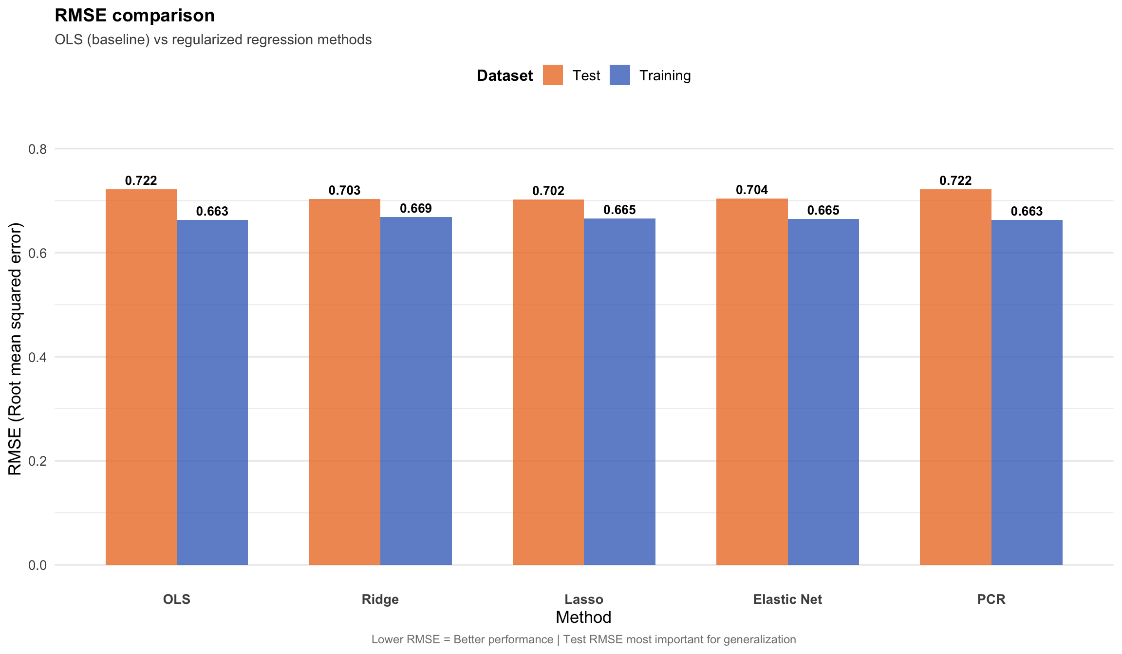
## RMSE comparison
```{r rmse-barplot}
#| label: fig-rmse-comparison
#| fig-cap: "RMSE comparison across all methods. Lower RMSE indicates better predictive performance. Regularized methods outperform vanilla OLS on test data."
#| fig-width: 12
#| fig-height: 7
#| code-summary: "Create RMSE comparison barplot"
rmse_comparison <- data.frame(
  Method = rep(c("OLS", "Ridge", "Lasso", "Elastic Net", "PCR"), 2),
  RMSE = c(comparison$Train_RMSE, comparison$Test_RMSE),
  Dataset = rep(c("Training", "Test"), each = 5)
)

rmse_comparison$Method <- factor(rmse_comparison$Method,
  levels = c("OLS", "Ridge", "Lasso", "Elastic Net",  "PCR")
)

p_rmse <- ggplot(rmse_comparison, aes(x = Method, y = RMSE, fill = Dataset)) +
  geom_col(position = "dodge", alpha = 0.8, width = 0.7) +
  geom_text(aes(label = sprintf("%.3f", RMSE)),
    position = position_dodge(width = 0.7),
    vjust = -0.5, size = 3.5, fontface = "bold"
  ) +
  scale_fill_manual(
    values = c("Training" = "#4472C4", "Test" = "#ED7D31"),
    name = "Dataset"
  ) +
  labs(
    title = "RMSE comparison",
    subtitle = "OLS (baseline) vs regularized regression methods",
    x = "Method",
    y = "RMSE (Root mean squared error)",
    caption = "Lower RMSE = Better performance | Test RMSE most important for generalization"
  ) +
  theme_minimal(base_size = 13) +
  theme(
    axis.text.x = element_text(angle = 0, hjust = 0.5, face = "bold"),
    legend.position = "top",
    legend.title = element_text(face = "bold", size = 12),
    legend.text = element_text(size = 11),
    plot.title = element_text(face = "bold", size = 14),
    plot.subtitle = element_text(size = 11, color = "gray30"),
    plot.caption = element_text(size = 9, color = "gray50", hjust = 0.5),
    panel.grid.major.x = element_blank()
  ) +
  ylim(0, max(rmse_comparison$RMSE) * 1.15)

p_rmse
```
```{r}
cat("\n=== RMSE Summary ===\n")
cat(
  "Best training RMSE:", comparison$Method[which.min(comparison$Train_RMSE)],
  "=", round(min(comparison$Train_RMSE), 4), "\n"
)
cat(
  "Best test RMSE:", comparison$Method[which.min(comparison$Test_RMSE)],
  "=", round(min(comparison$Test_RMSE), 4), "\n"
)
cat("\nTest RMSE improvement over OLS:\n")
for (i in 2:nrow(comparison)) {
  improvement <- ((ols_test_rmse - comparison$Test_RMSE[i]) / ols_test_rmse) * 100
  cat(sprintf("  %s: %.2f%% improvement\n", comparison$Method[i], improvement))
}
```
## Performance vis
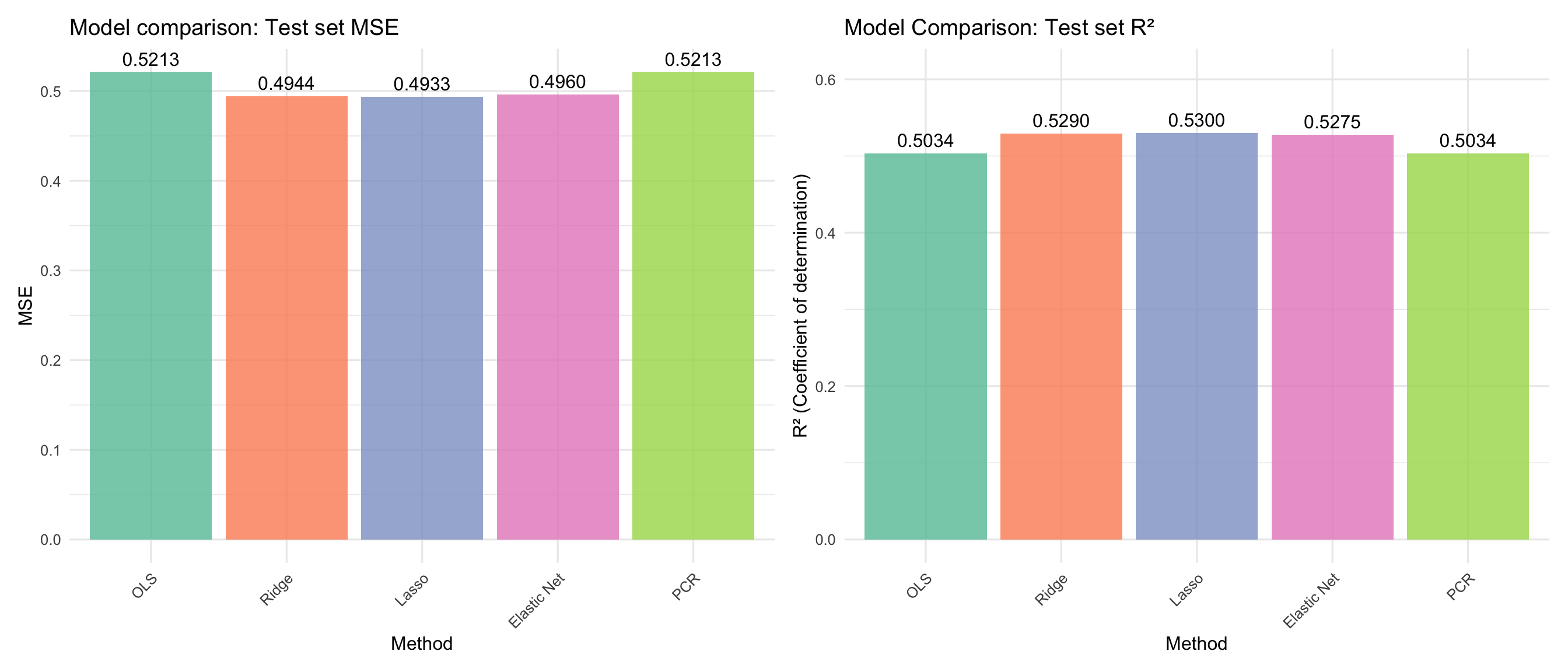
```{r comparison-viz}
#| label: fig-comparison
#| fig-cap: "Model comparison: Test set MSE and R² for all methods."
#| fig-width: 14
#| fig-height: 6
#| code-summary: "Create comparison plots"
comparison$Method <- factor(comparison$Method, levels = comparison$Method)

# Test MSE comparison
p_mse <- ggplot(comparison, aes(x = Method, y = Test_MSE, fill = Method)) +
  geom_col(alpha = 0.8) +
  geom_text(aes(label = sprintf("%.4f", Test_MSE)), vjust = -0.5) +
  scale_fill_brewer(palette = "Set2") +
  labs(
    title = "Model comparison: Test set MSE",
    x = "Method",
    y = "MSE"
  ) +
  theme_minimal(base_size = 12) +
  theme(
    legend.position = "none",
    axis.text.x = element_text(angle = 45, hjust = 1)
  )

# Test R² comparison
p_r2 <- ggplot(comparison, aes(x = Method, y = Test_R2, fill = Method)) +
  geom_col(alpha = 0.8) +
  geom_text(aes(label = sprintf("%.4f", Test_R2)), vjust = -0.5) +
  scale_fill_brewer(palette = "Set2") +
  labs(
    title = "Model Comparison: Test set R²",
    x = "Method",
    y = "R² (Coefficient of determination)"
  ) +
  ylim(0, max(comparison$Test_R2) * 1.15) +
  theme_minimal(base_size = 12) +
  theme(
    legend.position = "none",
    axis.text.x = element_text(angle = 45, hjust = 1)
  )

p_mse + p_r2
```
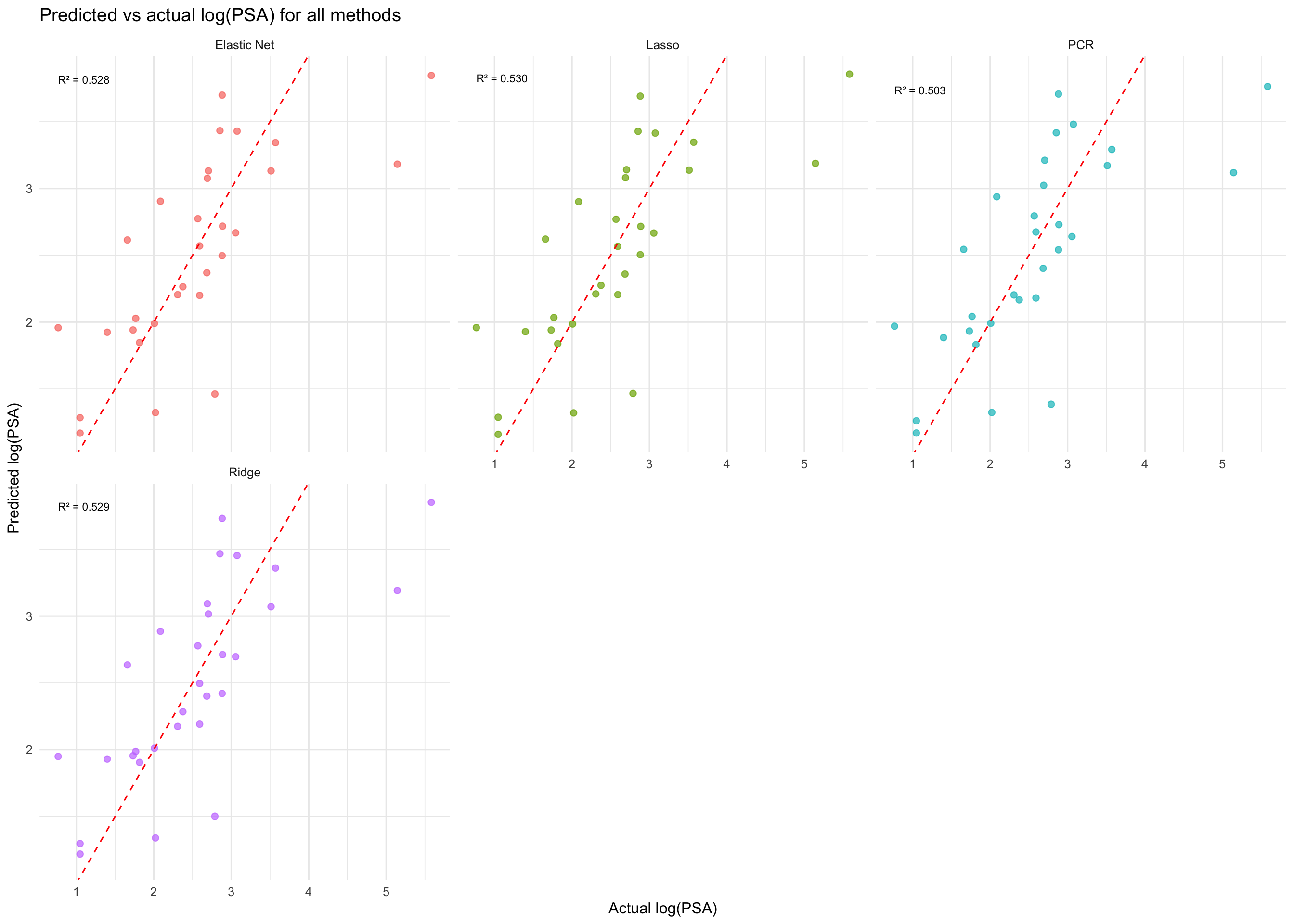
## Predicted vs actual
```{r pred-actual}
#| label: fig-pred-actual
#| fig-cap: "Predicted vs actual log(PSA) values for all five methods. Points close to the diagonal line indicate better predictions."
#| fig-width: 14
#| fig-height: 10
#| code-summary: "Create predicted vs actual plots"
pred_actual_df <- data.frame(
  Actual = rep(y_test, 4),
  Predicted = c(
    ridge_pred_test, lasso_pred_test, enet_pred_test,
    pcr_pred_test
  ),
  Method = rep(c("Ridge", "Lasso", "Elastic Net", "PCR"), each = length(y_test)),
  R2 = rep(c(ridge_test_r2, lasso_test_r2, enet_test_r2,  pcr_test_r2),
    each = length(y_test)
  )
)

ggplot(pred_actual_df, aes(x = Actual, y = Predicted)) +
  geom_point(aes(color = Method), size = 2, alpha = 0.7) +
  geom_abline(slope = 1, intercept = 0, linetype = "dashed", color = "red") +
  geom_text(
    data = pred_actual_df %>%
      group_by(Method, R2) %>%
      summarise(x = min(Actual), y = max(Predicted), .groups = "drop"),
    aes(x = x, y = y, label = sprintf("R² = %.3f", R2)),
    hjust = 0, vjust = 1, size = 3
  ) +
  facet_wrap(~Method, ncol = 3) +
  labs(
    title = "Predicted vs actual log(PSA) for all methods",
    x = "Actual log(PSA)",
    y = "Predicted log(PSA)"
  ) +
  theme_minimal(base_size = 12) +
  theme(legend.position = "none")
```
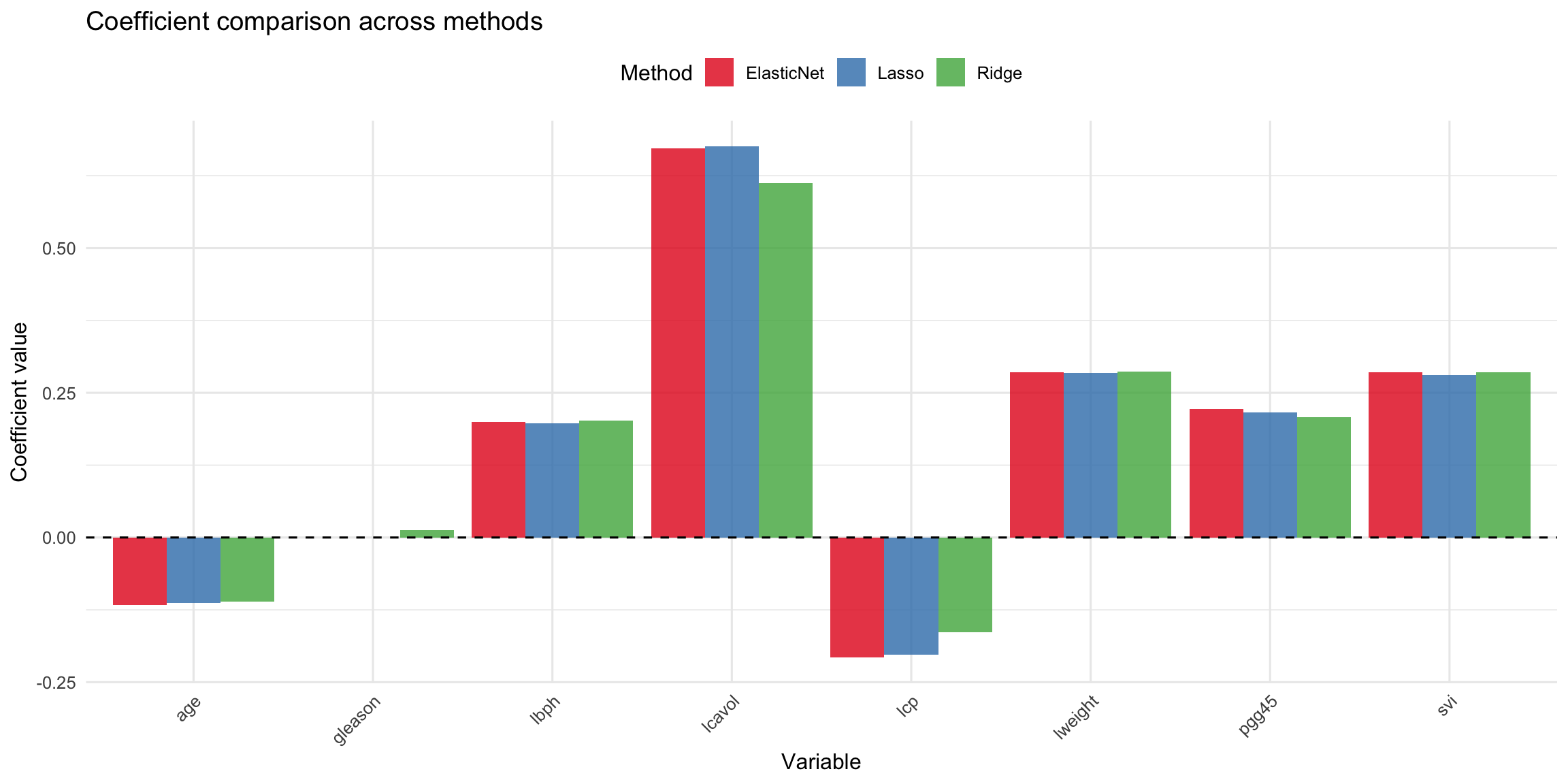
## Coefficient comparison
```{r coef-comparison}
#| label: fig-coef-comparison
#| fig-cap: "Coefficient values across ridge, lasso, and elastic net. Note how Lasso sets some coefficients to exactly zero."
#| fig-width: 12
#| fig-height: 6
#| code-summary: "Compare coefficients"
ridge_coef <- as.vector(coef(ridge_model))[-1]
lasso_coef <- as.vector(coef(lasso_model))[-1]
enet_coef <- as.vector(coef(enet_model))[-1]

coef_comparison <- data.frame(
  Variable = colnames(x_train),
  Ridge = ridge_coef,
  Lasso = lasso_coef,
  ElasticNet = enet_coef
)

coef_long <- pivot_longer(coef_comparison,
  cols = -Variable,
  names_to = "Method", values_to = "Coefficient"
)

ggplot(coef_long, aes(x = Variable, y = Coefficient, fill = Method)) +
  geom_col(position = "dodge", alpha = 0.8) +
  geom_hline(yintercept = 0, linetype = "dashed") +
  scale_fill_brewer(palette = "Set1") +
  labs(
    title = "Coefficient comparison across methods",
    x = "Variable",
    y = "Coefficient value"
  ) +
  theme_minimal(base_size = 12) +
  theme(
    axis.text.x = element_text(angle = 45, hjust = 1),
    legend.position = "top"
  )
```
::: {.callout-note icon=false appearance="simple"}
## Session info
```{r session-info}
#| echo: false
sessionInfo()
```
:::