Experiments with scVI

scvi-tools exists as a suite of tools for performing dimensionality reduction, data harmonization, and differential expression. One key advantage of using scvi-tools is that it inherently supports loading and training data in mini-batches and hence is practically infinitely scalable (Lopez et al., 2018).

scvi-tools uses generative modeling to model counts originating from a scRNA-seq experiment with different underlying models catering to other experiments. “Generative modeling” is a broad term that implies models of distributions $P(X)$ , defined over some collection of datapoints $X$ that exist in a high dimensional space. In scRNA-seq, each datapoint corresponds to a cell $c$ which has a multidimensional vector $X_{c,g} \in \mathcal{R}^{20000}$ containing read counts or UMIs of 20000 genes. A scRNA-seq datasets contains not one but a few thousand if not millions of cells. The generative model’s task is to capture the underlying representation of these cells. “Representation” here is a loose term, but more formally given a $\text{gene} \times \text{cell}$ matrix whose distribution $P_{\text{truth}}(X)$ is unknown, the generative model tries to learn a distribution $P(X)$ which is as close to $P_{\text{truth}}(X)$ as possible.

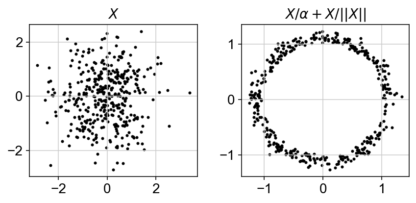
In order to obtain $P(X)$ , the model should be able to exploit the underlying structure in data. Neural networks are powerful functional approximators given their ability to capture non-linearities. Variational autoencoders utilize neural networks to build generative models that can approximate $P_{truth}(X)$ in a decently quick fashion. The reason this works is because any $d$ dimensional distribution can be approximated by starting with $d$ gaussian random variables and passing them through a complicated function (Devroye, 1986). A famous example of this is generating a 2D circle from a 2D gaussian blob.

Figure 1. A 2D gaussian blob can be passed through a sufficiently complicated function $g(z) = \frac{z}{\alpha} + \frac{z}{||z||}$ to obtain a 2D ring.

scvi-tools also starts from a gaussian random variable and propogates it through its various layers such that the output count for a gene and a particular cells is close to its observed value. It does it over four main steps:

1. Generate a gaussian

2. Pass the gaussian through a neural network to approximate gene-cell proportions ($\rho_{g,c}$)

3. Generate a count $y_{c,g}$ for each gene-cell using the estimated proportion in step 2 and and the total sequencing depth along with an estimated dispersion $\phi_g$.

4. Calculate reconstruction error between generated count $y_{c,g}$ and observed count $x_{c,g}$

The aim is to minimize the reconstruction error in step 4 by optimizing the neural network weights and the estimated parameters $\rho_{c,g}$ and $\theta_g$.

$\begin{aligned} {\color{purple}z_c} &\sim \mathcal{N}(0,I) & \text{\color{purple}Cell embedding} \\ {\color{red}\rho_{g,c}} &\sim \text{softmax}(f_w(z_c)) & \text{\color{red}Normalized expression } \\ y_{c,g} &\sim \text{NB}({\color{blue} l_c} {\color{red}\rho_{c,g}}, \phi_g) & \text{Observed counts} \end{aligned}$

The total sequencing depth for a cell can be also be learned by the network inherently, but the latest version (0.8.0) of scVI supports using observed library size. I started using observed library sizes before it became part of the implementation. The training time is faster and in my limited testing, the downstream clustering results look slightly better with using observed library size, but it could also be due to other reasons.

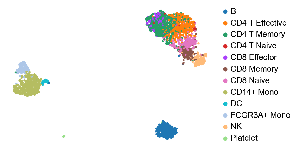
The latent distribution $Z$ thus learned is a reduced dimensional latent reprsentation of the data. I will use [PBMC3k dataset] (https://support.10xgenomics.com/single-cell-gene-expression/datasets/1.1.0/pbmc3k) for all the analysis here. We can do a UMAP visualization and the clusters tend to match up pretty well with ground truth, though there is possiblity of improvement.

Figure 1. UMAP on the latent representation learned by scvi on PBMC3k dataset.

We now have a $P(Y)$ and access to all intermediate values we can do a ton of things. But the first thing would be to check if $P(Y)$ is indeed correct. One such way of performing validity checks on this model is posterior predictive checks (PPC). I learned of PPCs through Richard McElreath’s Statistical Rethinking (McElreath, 2020), which forms an integral part of all his discussions.

The idea of a PPC is very simple: simulate replicate data from the learned model and compare it to the observed. In a way you are using your data twice, to learn the model and then using the learned model to check it against the same data. A better designed check would be done on held out dataset, but it is perfectly valid to test the model against the observations used to train the model.

The simplest checks for scRNA-seq counts is the mean-variance relationships. The simulated means and variances from the learned model should match that of the observed data on both a cell and a gene level.

Figure 2. Comparison of generated against observed means, variance and mean-variance relationships.

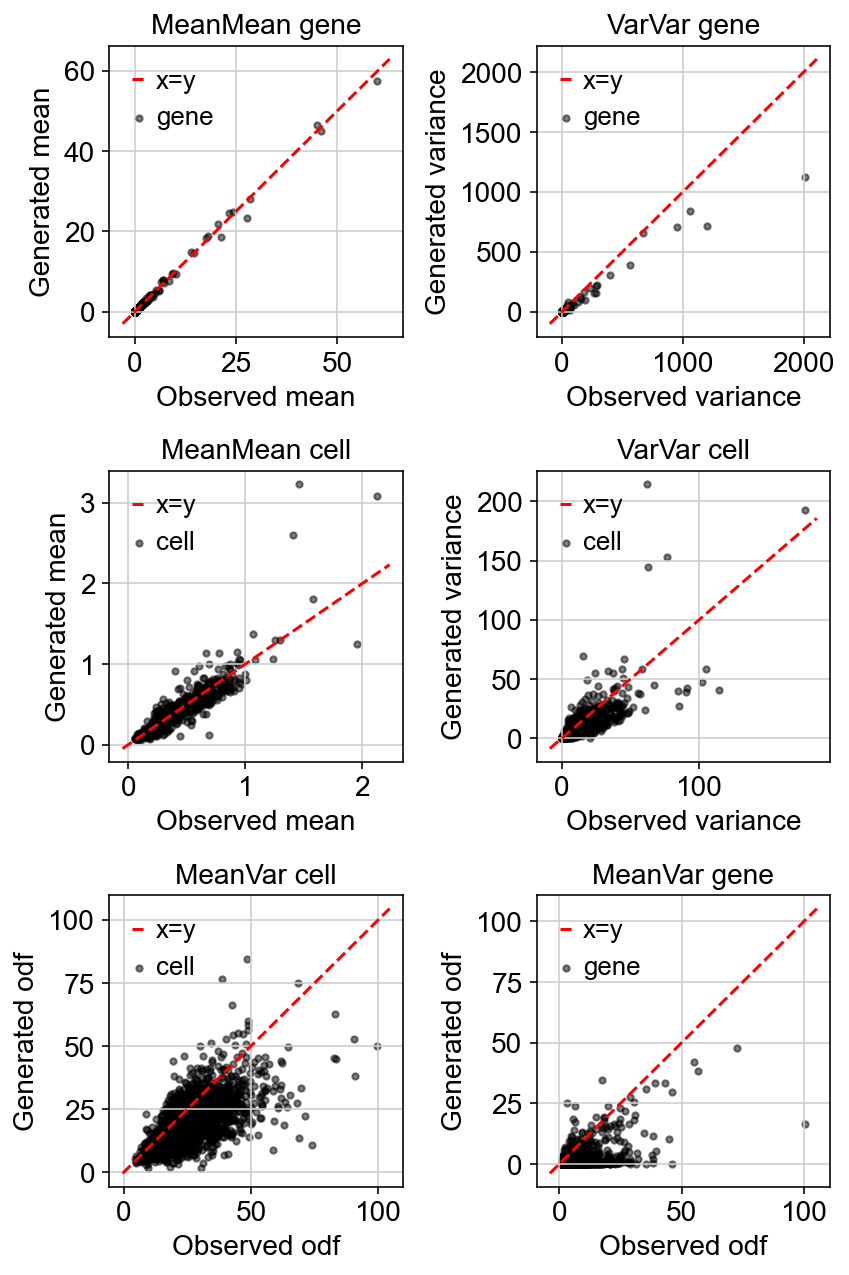
The simulated mean-variance relationship aligns very well with the observed relationship.

Let’s compare how the dispersion looks like:

Figure 3. Comparison of generated against observed means, variance and mean-variance.

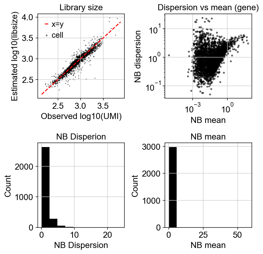
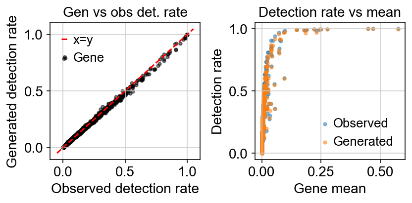
Variation with gene detection rate:

Figure 4. Comparison of generated against observed means, variance and mean-variance.

The loss function being minizmied to infere the parameters minimizes the reconstruction loss between generated counts $X$ and observed counts $Y$.

Figure 5. Comparison of generated against observed means, variance and mean-variance.

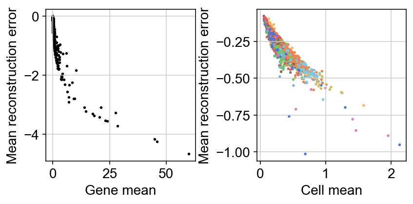
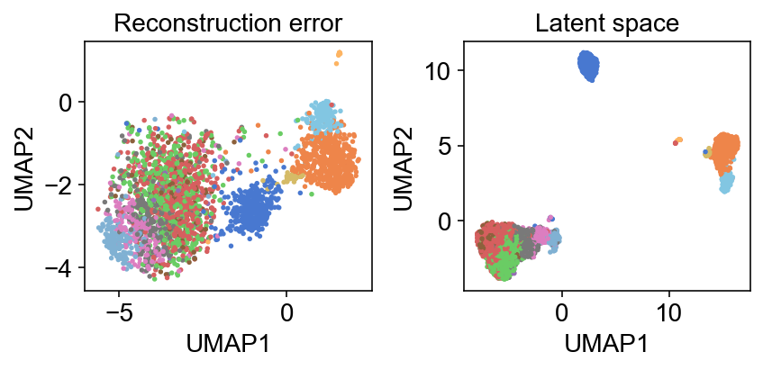
One thing I still need to wrap around my head is how much informative the reconstruction error itself is. For example, a UMAP of this reconstruction error mimics that of the latent representation:

Figure 5. Comparison of generated against observed means, variance and mean-variance.

1. Lopez, R., Regier, J., Cole, M. B., Jordan, M. I., & Yosef, N. (2018). Deep generative modeling for single-cell transcriptomics. Nature Methods, 15(12), 1053–1058.
2. Devroye, L. (1986). Sample-based non-uniform random variate generation. Proceedings of the 18th Conference on Winter Simulation, 260–265.
3. McElreath, R. (2020). Statistical rethinking: A Bayesian course with examples in R and Stan. CRC press.
4. Ma, S., Zhang, B., LaFave, L. M., Earl, A. S., Chiang, Z., Hu, Y., Ding, J., Brack, A., Kartha, V. K., Tay, T., & others. (2020). Chromatin potential identified by shared single-cell profiling of RNA and chromatin. Cell, 183(4), 1103–1116.