![]()
1. Chapter 1 - Introduction to Linear and Generalized Linear Models
import warnings

import pandas as pd
import proplot as plot
import seaborn as sns
import statsmodels.api as sm
import statsmodels.formula.api as smf
from patsy import dmatrices
from scipy import stats

warnings.filterwarnings("ignore")
%pylab inline


plt.rcParams["axes.labelweight"] = "bold"
plt.rcParams["font.weight"] = "bold"
/opt/hostedtoolcache/Python/3.7.9/x64/lib/python3.7/site-packages/proplot/config.py:1454: ProPlotWarning: Rebuilding font cache.
Populating the interactive namespace from numpy and matplotlib
crabs_df = pd.read_csv("../data/Crabs.tsv.gz", sep="\t")
crabs_df.head()
| crab | y | weight | width | color | spine | |
|---|---|---|---|---|---|---|
| 1 | 1 | 8 | 3.05 | 28.3 | 2 | 3 |
| 2 | 2 | 0 | 1.55 | 22.5 | 3 | 3 |
| 3 | 3 | 9 | 2.30 | 26.0 | 1 | 1 |
| 4 | 4 | 0 | 2.10 | 24.8 | 3 | 3 |
| 5 | 5 | 4 | 2.60 | 26.0 | 3 | 3 |
This data comes from a study of female horseshoe crabs (citation unknown). During spawning session, the females migrate to the shore to brred. The males then attach themselves to females’ posterior spine while the females burrows into the sand and lays cluster of eggs. The fertilization of eggs happens externally in the sand beneath the pair. During this spanwing, multulpe males may cluster the pair and may also fertilize the eggs. These males are called satellites.
crab: observation index
y: Number of satellites attached
weight: weight of the female crab
color: color of the female
spine:condition of female’s spine
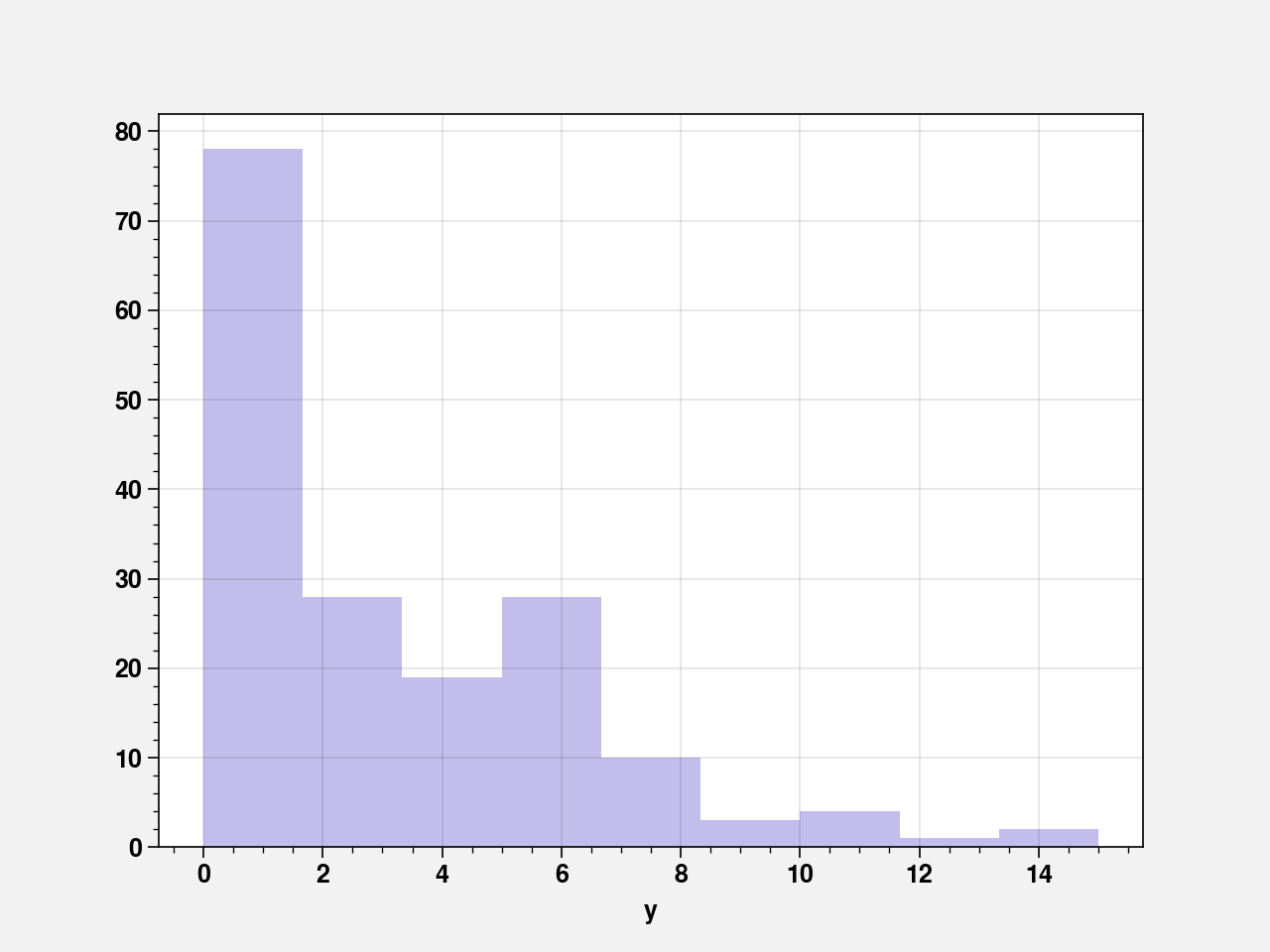
print((crabs_df["y"].mean(), crabs_df["y"].var()))
(2.9190751445086707, 9.912017744320472)
sns.distplot(crabs_df["y"], kde=False, color="slateblue")
<AxesSubplot:xlabel='y'>
pd.crosstab(index=crabs_df["y"], columns="count")
| col_0 | count |
|---|---|
| y | |
| 0 | 62 |
| 1 | 16 |
| 2 | 9 |
| 3 | 19 |
| 4 | 19 |
| 5 | 15 |
| 6 | 13 |
| 7 | 4 |
| 8 | 6 |
| 9 | 3 |
| 10 | 3 |
| 11 | 1 |
| 12 | 1 |
| 14 | 1 |
| 15 | 1 |
formula = """y ~ 1"""
response, predictors = dmatrices(formula, crabs_df, return_type="dataframe")
fit_pois = sm.GLM(
    response, predictors, family=sm.families.Poisson(link=sm.families.links.identity())
).fit()
print(fit_pois.summary())
                 Generalized Linear Model Regression Results
==============================================================================
Dep. Variable:                      y   No. Observations:                  173
Model:                            GLM   Df Residuals:                      172
Model Family:                 Poisson   Df Model:                            0
Link Function:               identity   Scale:                          1.0000
Method:                          IRLS   Log-Likelihood:                -494.04
Date:                Tue, 12 Jan 2021   Deviance:                       632.79
Time:                        23:01:17   Pearson chi2:                     584.
No. Iterations:                     3
Covariance Type:            nonrobust
==============================================================================
                 coef    std err          z      P>|z|      [0.025      0.975]
------------------------------------------------------------------------------
Intercept      2.9191      0.130     22.472      0.000       2.664       3.174
==============================================================================
Fitting a Poisson distribution with a GLM containing only an iontercept and using identity link function gives the estimate of intercept which is essentially the mean of y. But poisson has the same mean as its variance. The sample variance of 9.92 suggests that a poisson fit is not appropriate here.
1.1. Linear Model Using Weight to Predict Satellite Counts
print((crabs_df["weight"].mean(), crabs_df["weight"].var()))
(2.437190751445087, 0.33295809712326924)
print(crabs_df["weight"].quantile(q=[0, 0.25, 0.5, 0.75, 1]))
0.00    1.20
0.25    2.00
0.50    2.35
0.75    2.85
1.00    5.20
Name: weight, dtype: float64
fig, ax = plt.subplots(figsize=(5, 5))
ax.scatter(crabs_df["weight"], crabs_df["y"])
ax.set_xlabel("weight")
ax.set_ylabel("y")
Text(0, 0.5, 'y')
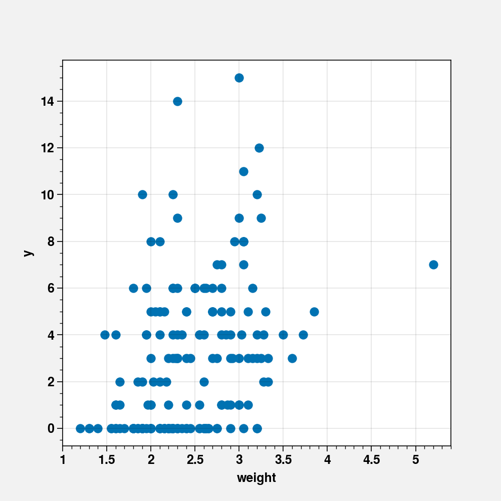
The plot shows that there is no clear trend in relation between y (number of satellites) and weight.
1.2. Fit a LM vs GLM (Gaussian)
formula = """y ~ weight"""
fit_weight = smf.ols(formula=formula, data=crabs_df).fit()
print(fit_weight.summary())
                            OLS Regression Results
==============================================================================
Dep. Variable:                      y   R-squared:                       0.136
Model:                            OLS   Adj. R-squared:                  0.131
Method:                 Least Squares   F-statistic:                     27.00
Date:                Tue, 12 Jan 2021   Prob (F-statistic):           5.75e-07
Time:                        23:01:17   Log-Likelihood:                -430.70
No. Observations:                 173   AIC:                             865.4
Df Residuals:                     171   BIC:                             871.7
Df Model:                           1
Covariance Type:            nonrobust
==============================================================================
                 coef    std err          t      P>|t|      [0.025      0.975]
------------------------------------------------------------------------------
Intercept     -1.9911      0.971     -2.050      0.042      -3.908      -0.074
weight         2.0147      0.388      5.196      0.000       1.249       2.780
==============================================================================
Omnibus:                       38.273   Durbin-Watson:                   1.750
Prob(Omnibus):                  0.000   Jarque-Bera (JB):               58.768
Skew:                           1.188   Prob(JB):                     1.73e-13
Kurtosis:                       4.584   Cond. No.                         12.6
==============================================================================

Notes:
[1] Standard Errors assume that the covariance matrix of the errors is correctly specified.
response, predictors = dmatrices(formula, crabs_df, return_type="dataframe")
fit_weight2 = sm.GLM(response, predictors, family=sm.families.Gaussian()).fit()
print(fit_weight2.summary())
                 Generalized Linear Model Regression Results
==============================================================================
Dep. Variable:                      y   No. Observations:                  173
Model:                            GLM   Df Residuals:                      171
Model Family:                Gaussian   Df Model:                            1
Link Function:               identity   Scale:                          8.6106
Method:                          IRLS   Log-Likelihood:                -430.70
Date:                Tue, 12 Jan 2021   Deviance:                       1472.4
Time:                        23:01:17   Pearson chi2:                 1.47e+03
No. Iterations:                     3
Covariance Type:            nonrobust
==============================================================================
                 coef    std err          z      P>|z|      [0.025      0.975]
------------------------------------------------------------------------------
Intercept     -1.9911      0.971     -2.050      0.040      -3.894      -0.088
weight         2.0147      0.388      5.196      0.000       1.255       2.775
==============================================================================
Thus OLS and a GLM using Gaussian family and identity link are one and the same.
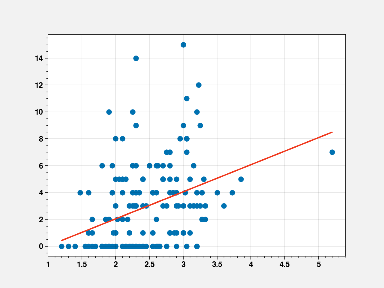
1.3. Plotting the linear fit
fig, ax = plt.subplots()
ax.scatter(crabs_df["weight"], crabs_df["y"])
line = fit_weight2.params[0] + fit_weight2.params[1] * crabs_df["weight"]

ax.plot(crabs_df["weight"], line, color="#f03b20")
[<matplotlib.lines.Line2D at 0x7f37426eff10>]
1.4. Comparing Mean Numbers of Satellites by Crab Color
crabs_df["color"].value_counts()
2    95
3    44
4    22
1    12
Name: color, dtype: int64
color: 1 = medium light, 2 = medium, 3 = medium dark, 4 = dark
crabs_df.groupby("color").agg(["mean", "var"])[["y"]]
| y | ||
|---|---|---|
| mean | var | |
| color | ||
| 1 | 4.083333 | 9.719697 |
| 2 | 3.294737 | 10.273908 |
| 3 | 2.227273 | 6.737844 |
| 4 | 2.045455 | 13.093074 |
Majority of the crabs are of medoum color and the mean response also decreases as the color gets darker.
If we fit a linear model between \(y\) and \(color\) using sm.ols, color is treated as a quantitative variable:
mod = smf.ols(formula="y ~ color", data=crabs_df)
res = mod.fit()
print(res.summary())
                            OLS Regression Results
==============================================================================
Dep. Variable:                      y   R-squared:                       0.036
Model:                            OLS   Adj. R-squared:                  0.031
Method:                 Least Squares   F-statistic:                     6.459
Date:                Tue, 12 Jan 2021   Prob (F-statistic):             0.0119
Time:                        23:01:17   Log-Likelihood:                -440.18
No. Observations:                 173   AIC:                             884.4
Df Residuals:                     171   BIC:                             890.7
Df Model:                           1
Covariance Type:            nonrobust
==============================================================================
                 coef    std err          t      P>|t|      [0.025      0.975]
------------------------------------------------------------------------------
Intercept      4.7461      0.757      6.274      0.000       3.253       6.239
color         -0.7490      0.295     -2.542      0.012      -1.331      -0.167
==============================================================================
Omnibus:                       38.876   Durbin-Watson:                   1.780
Prob(Omnibus):                  0.000   Jarque-Bera (JB):               59.793
Skew:                           1.207   Prob(JB):                     1.04e-13
Kurtosis:                       4.570   Cond. No.                         9.39
==============================================================================

Notes:
[1] Standard Errors assume that the covariance matrix of the errors is correctly specified.
Let’s treat color as a qualitative variable:
mod = smf.ols(formula="y ~ C(color)", data=crabs_df)
res = mod.fit()
print(res.summary())
                            OLS Regression Results
==============================================================================
Dep. Variable:                      y   R-squared:                       0.040
Model:                            OLS   Adj. R-squared:                  0.023
Method:                 Least Squares   F-statistic:                     2.323
Date:                Tue, 12 Jan 2021   Prob (F-statistic):             0.0769
Time:                        23:01:17   Log-Likelihood:                -439.89
No. Observations:                 173   AIC:                             887.8
Df Residuals:                     169   BIC:                             900.4
Df Model:                           3
Covariance Type:            nonrobust
=================================================================================
                    coef    std err          t      P>|t|      [0.025      0.975]
---------------------------------------------------------------------------------
Intercept         4.0833      0.899      4.544      0.000       2.310       5.857
C(color)[T.2]    -0.7886      0.954     -0.827      0.409      -2.671       1.094
C(color)[T.3]    -1.8561      1.014     -1.831      0.069      -3.857       0.145
C(color)[T.4]    -2.0379      1.117     -1.824      0.070      -4.243       0.167
==============================================================================
Omnibus:                       37.294   Durbin-Watson:                   1.779
Prob(Omnibus):                  0.000   Jarque-Bera (JB):               55.871
Skew:                           1.179   Prob(JB):                     7.38e-13
Kurtosis:                       4.479   Cond. No.                         9.31
==============================================================================

Notes:
[1] Standard Errors assume that the covariance matrix of the errors is correctly specified.
This is equivalent to doing a GLM fit with a gaussian family and identity link:
formula = """y ~ C(color)"""
response, predictors = dmatrices(formula, crabs_df, return_type="dataframe")
fit_color = sm.GLM(response, predictors, family=sm.families.Gaussian()).fit()
print(fit_color.summary())
                 Generalized Linear Model Regression Results
==============================================================================
Dep. Variable:                      y   No. Observations:                  173
Model:                            GLM   Df Residuals:                      169
Model Family:                Gaussian   Df Model:                            3
Link Function:               identity   Scale:                          9.6884
Method:                          IRLS   Log-Likelihood:                -439.89
Date:                Tue, 12 Jan 2021   Deviance:                       1637.3
Time:                        23:01:18   Pearson chi2:                 1.64e+03
No. Iterations:                     3
Covariance Type:            nonrobust
=================================================================================
                    coef    std err          z      P>|z|      [0.025      0.975]
---------------------------------------------------------------------------------
Intercept         4.0833      0.899      4.544      0.000       2.322       5.844
C(color)[T.2]    -0.7886      0.954     -0.827      0.408      -2.658       1.080
C(color)[T.3]    -1.8561      1.014     -1.831      0.067      -3.843       0.131
C(color)[T.4]    -2.0379      1.117     -1.824      0.068      -4.227       0.151
=================================================================================
If we instead do a poisson fit:
formula = """y ~ C(color)"""
response, predictors = dmatrices(formula, crabs_df, return_type="dataframe")
fit_color2 = sm.GLM(
    response, predictors, family=sm.families.Poisson(link=sm.families.links.identity)
).fit()
print(fit_color2.summary())
                 Generalized Linear Model Regression Results
==============================================================================
Dep. Variable:                      y   No. Observations:                  173
Model:                            GLM   Df Residuals:                      169
Model Family:                 Poisson   Df Model:                            3
Link Function:               identity   Scale:                          1.0000
Method:                          IRLS   Log-Likelihood:                -482.22
Date:                Tue, 12 Jan 2021   Deviance:                       609.14
Time:                        23:01:18   Pearson chi2:                     584.
No. Iterations:                     3
Covariance Type:            nonrobust
=================================================================================
                    coef    std err          z      P>|z|      [0.025      0.975]
---------------------------------------------------------------------------------
Intercept         4.0833      0.583      7.000      0.000       2.940       5.227
C(color)[T.2]    -0.7886      0.612     -1.288      0.198      -1.989       0.412
C(color)[T.3]    -1.8561      0.625     -2.969      0.003      -3.081      -0.631
C(color)[T.4]    -2.0379      0.658     -3.096      0.002      -3.328      -0.748
=================================================================================
And we get the same estimates as when using Gaussian family with identity link! Because the ML estimates for the poisson distirbution is also the sample mean if there is a single predictor. But the standard values are much smaller. Because the errors here are heteroskedastic while the gaussian version assume homoskesdasticity.
1.5. Using both qualitative and quantitative variables
formula = """y ~ weight + C(color)"""
response, predictors = dmatrices(formula, crabs_df, return_type="dataframe")
fit_weight_color = sm.GLM(response, predictors, family=sm.families.Gaussian()).fit()
print(fit_weight_color.summary())
                 Generalized Linear Model Regression Results
==============================================================================
Dep. Variable:                      y   No. Observations:                  173
Model:                            GLM   Df Residuals:                      168
Model Family:                Gaussian   Df Model:                            4
Link Function:               identity   Scale:                          8.6370
Method:                          IRLS   Log-Likelihood:                -429.44
Date:                Tue, 12 Jan 2021   Deviance:                       1451.0
Time:                        23:01:18   Pearson chi2:                 1.45e+03
No. Iterations:                     3
Covariance Type:            nonrobust
=================================================================================
                    coef    std err          z      P>|z|      [0.025      0.975]
---------------------------------------------------------------------------------
Intercept        -0.8232      1.355     -0.608      0.543      -3.479       1.832
C(color)[T.2]    -0.6181      0.901     -0.686      0.493      -2.384       1.148
C(color)[T.3]    -1.2404      0.966     -1.284      0.199      -3.134       0.653
C(color)[T.4]    -1.1882      1.070     -1.110      0.267      -3.286       0.910
weight            1.8662      0.402      4.645      0.000       1.079       2.654
=================================================================================
formula = """y ~ weight + C(color)"""
response, predictors = dmatrices(formula, crabs_df, return_type="dataframe")
fit_weight_color2 = sm.GLM(
    response, predictors, family=sm.families.Poisson(link=sm.families.links.identity())
).fit()
print(fit_weight_color2.summary())
                 Generalized Linear Model Regression Results
==============================================================================
Dep. Variable:                      y   No. Observations:                  173
Model:                            GLM   Df Residuals:                      168
Model Family:                 Poisson   Df Model:                            4
Link Function:               identity   Scale:                          1.0000
Method:                          IRLS   Log-Likelihood:                    nan
Date:                Tue, 12 Jan 2021   Deviance:                       534.33
Time:                        23:01:18   Pearson chi2:                     529.
No. Iterations:                   100
Covariance Type:            nonrobust
=================================================================================
                    coef    std err          z      P>|z|      [0.025      0.975]
---------------------------------------------------------------------------------
Intercept        -0.9930      0.736     -1.349      0.177      -2.436       0.450
C(color)[T.2]    -0.8442      0.615     -1.374      0.170      -2.049       0.360
C(color)[T.3]    -1.4320      0.629     -2.278      0.023      -2.664      -0.200
C(color)[T.4]    -1.2248      0.658     -1.861      0.063      -2.515       0.065
weight            2.0086      0.173     11.641      0.000       1.670       2.347
=================================================================================