![]()
2. Chapter 2 - Linear Models: Least Squares Theory
import warnings

import pandas as pd
import proplot as plot
import seaborn as sns
import statsmodels.api as sm
import statsmodels.formula.api as smf
from patsy import dmatrices
from scipy import stats

warnings.filterwarnings("ignore")
%pylab inline


plt.rcParams["axes.labelweight"] = "bold"
plt.rcParams["font.weight"] = "bold"
Populating the interactive namespace from numpy and matplotlib
scots_races_df = pd.read_csv("../data/ScotsRaces.tsv.gz", sep="\t")
scots_races_df.head()
| race | distance | climb | time | |
|---|---|---|---|---|
| 1 | GreenmantleNewYearDash | 2.5 | 0.65 | 16.08 |
| 2 | Carnethy5HillRace | 6.0 | 2.50 | 48.35 |
| 3 | CraigDunainHillRace | 6.0 | 0.90 | 33.65 |
| 4 | BenRhaHillRace | 7.5 | 0.80 | 45.60 |
| 5 | BenLomondHillRace | 8.0 | 3.07 | 62.27 |
A dataset contains a list of hill races in Scotland for the year. Explanatory variables:
distance of the race (in miles)
the cumulative climb (in thousands of feet)
print(scots_races_df[["time", "climb", "distance"]].mean(axis=0))
print(scots_races_df[["time", "climb", "distance"]].std(axis=0))
time        56.089714
climb        1.815314
distance     7.528571
dtype: float64
time        50.392617
climb        1.619151
distance     5.523936
dtype: float64
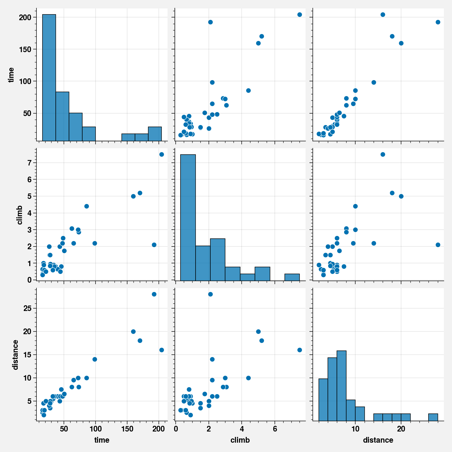
sns.pairplot(scots_races_df[["time", "climb", "distance"]])
<seaborn.axisgrid.PairGrid at 0x7f14f9889510>
scots_races_df[["climb", "distance", "time"]].corr()
| climb | distance | time | |
|---|---|---|---|
| climb | 1.000000 | 0.652346 | 0.832654 |
| distance | 0.652346 | 1.000000 | 0.943094 |
| time | 0.832654 | 0.943094 | 1.000000 |
fit_cd = smf.ols(
    formula="""time ~ climb + distance""",
    data=scots_races_df[["climb", "distance", "time"]],
).fit()
print(fit_cd.summary())
                            OLS Regression Results
==============================================================================
Dep. Variable:                   time   R-squared:                       0.972
Model:                            OLS   Adj. R-squared:                  0.970
Method:                 Least Squares   F-statistic:                     549.9
Date:                Tue, 12 Jan 2021   Prob (F-statistic):           1.67e-25
Time:                        23:01:23   Log-Likelihood:                -123.95
No. Observations:                  35   AIC:                             253.9
Df Residuals:                      32   BIC:                             258.6
Df Model:                           2
Covariance Type:            nonrobust
==============================================================================
                 coef    std err          t      P>|t|      [0.025      0.975]
------------------------------------------------------------------------------
Intercept    -13.1086      2.561     -5.119      0.000     -18.325      -7.892
climb         11.7801      1.221      9.651      0.000       9.294      14.266
distance       6.3510      0.358     17.751      0.000       5.622       7.080
==============================================================================
Omnibus:                        7.207   Durbin-Watson:                   1.983
Prob(Omnibus):                  0.027   Jarque-Bera (JB):                6.967
Skew:                           0.598   Prob(JB):                       0.0307
Kurtosis:                       4.829   Cond. No.                         16.7
==============================================================================

Notes:
[1] Standard Errors assume that the covariance matrix of the errors is correctly specified.
Thus, adjusted for climb, the predicted record time increased by 6.34 minutes for every additional midle of distance
sns.distplot(fit_cd.resid, kde=False, color="slateblue")
<AxesSubplot:>
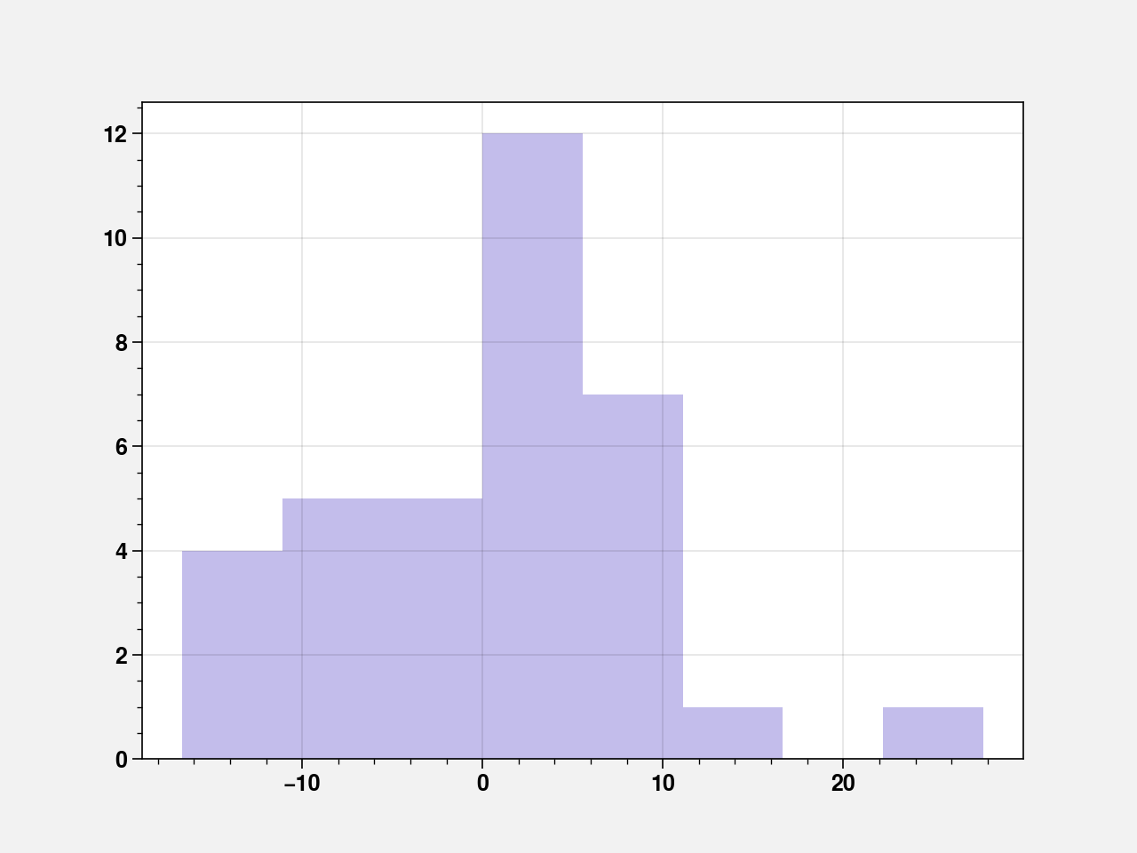
pd.Series(fit_cd.resid_pearson).quantile(q=[0, 0.25, 0.5, 0.75, 1])
0.00   -1.906667
0.25   -0.554349
0.50    0.127085
0.75    0.534341
1.00    3.178498
dtype: float64
print(stats.pearsonr(fit_cd.fittedvalues, fit_cd.resid))
(3.755818658506266e-15, 0.9999999999999806)
print(fit_cd.resid_pearson.mean(), fit_cd.resid_pearson.std())
6.483702463810914e-15 0.9561828874675148
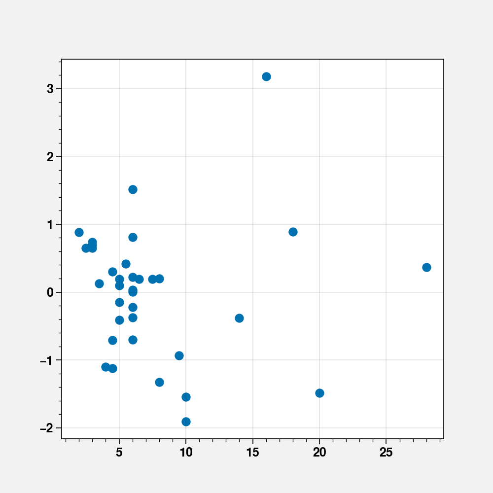
fig, ax = plt.subplots(figsize=(5, 5))
ax.scatter(scots_races_df["distance"], fit_cd.resid_pearson)
<matplotlib.collections.PathCollection at 0x7f14f0e6b650>
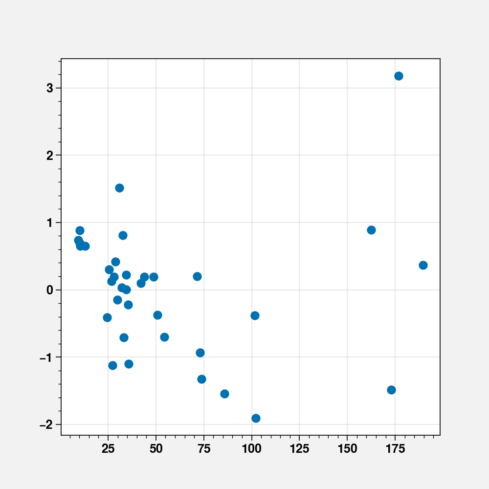
fig, ax = plt.subplots(figsize=(5, 5))
ax.scatter(fit_cd.fittedvalues, fit_cd.resid_pearson)
<matplotlib.collections.PathCollection at 0x7f14ee9f5710>
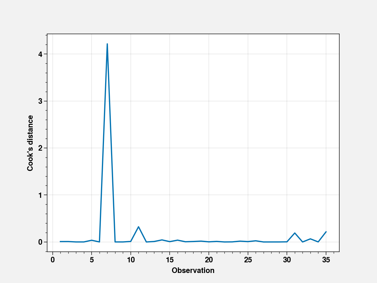
influence = fit_cd.get_influence()
summary_frame = influence.summary_frame()
fig, ax = plt.subplots()
ax.plot(summary_frame["cooks_d"])
ax.set_xlabel("Observation")
ax.set_ylabel("Cook's distance")
Text(0, 0.5, "Cook's distance")
2.1. ANOVA
lm = smf.ols(
    formula="""time ~ climb + distance""",
    data=scots_races_df[["climb", "distance", "time"]],
).fit()
table = sm.stats.anova_lm(lm, typ=2)
print(table)
                sum_sq    df           F        PR(>F)
climb      7105.618848   1.0   93.139930  5.368815e-11
distance  24038.225642   1.0  315.091296  3.990140e-18
Residual   2441.270928  32.0         NaN           NaN
# Change order
lm = smf.ols(
    formula="""time ~ distance + climb""",
    data=scots_races_df[["climb", "distance", "time"]],
).fit()
table = sm.stats.anova_lm(lm, typ=2)
print(table)
                sum_sq    df           F        PR(>F)
distance  24038.225642   1.0  315.091296  3.990140e-18
climb      7105.618848   1.0   93.139930  5.368815e-11
Residual   2441.270928  32.0         NaN           NaN
lm = smf.ols(
    formula="""time ~ climb + distance + climb:distance """,
    data=scots_races_df[["climb", "distance", "time"]],
).fit()
table = sm.stats.anova_lm(lm, typ=2)
print(lm.summary())
                            OLS Regression Results
==============================================================================
Dep. Variable:                   time   R-squared:                       0.981
Model:                            OLS   Adj. R-squared:                  0.979
Method:                 Least Squares   F-statistic:                     524.1
Date:                Tue, 12 Jan 2021   Prob (F-statistic):           1.24e-26
Time:                        23:01:24   Log-Likelihood:                -117.30
No. Observations:                  35   AIC:                             242.6
Df Residuals:                      31   BIC:                             248.8
Df Model:                           3
Covariance Type:            nonrobust
==================================================================================
                     coef    std err          t      P>|t|      [0.025      0.975]
----------------------------------------------------------------------------------
Intercept         -0.7672      3.906     -0.196      0.846      -8.733       7.199
climb              3.7133      2.365      1.570      0.126      -1.110       8.536
distance           4.9623      0.474     10.464      0.000       3.995       5.929
climb:distance     0.6598      0.174      3.786      0.001       0.304       1.015
==============================================================================
Omnibus:                        9.175   Durbin-Watson:                   1.509
Prob(Omnibus):                  0.010   Jarque-Bera (JB):               14.024
Skew:                          -0.486   Prob(JB):                     0.000901
Kurtosis:                       5.945   Cond. No.                         128.
==============================================================================

Notes:
[1] Standard Errors assume that the covariance matrix of the errors is correctly specified.