![]()
4. Chapter 4 - Generalized Linear Models: Model Fitting and Inference
import warnings

import pandas as pd
import proplot as plot
import seaborn as sns
import statsmodels.api as sm
import statsmodels.formula.api as smf
from patsy import dmatrices
from scipy import stats

warnings.filterwarnings("ignore")
%pylab inline


plt.rcParams["axes.labelweight"] = "bold"
plt.rcParams["font.weight"] = "bold"
Populating the interactive namespace from numpy and matplotlib
crabs_df = pd.read_csv("../data/Crabs.tsv.gz", sep="\t")
crabs_df.head()
| crab | y | weight | width | color | spine | |
|---|---|---|---|---|---|---|
| 1 | 1 | 8 | 3.05 | 28.3 | 2 | 3 |
| 2 | 2 | 0 | 1.55 | 22.5 | 3 | 3 |
| 3 | 3 | 9 | 2.30 | 26.0 | 1 | 1 |
| 4 | 4 | 0 | 2.10 | 24.8 | 3 | 3 |
| 5 | 5 | 4 | 2.60 | 26.0 | 3 | 3 |
formula = """y ~ width"""
response, predictors = dmatrices(formula, crabs_df, return_type="dataframe")
fit = sm.GLM(
    response, predictors, family=sm.families.Poisson(link=sm.families.links.log())
).fit()
print(fit.summary())
                 Generalized Linear Model Regression Results
==============================================================================
Dep. Variable:                      y   No. Observations:                  173
Model:                            GLM   Df Residuals:                      171
Model Family:                 Poisson   Df Model:                            1
Link Function:                    log   Scale:                          1.0000
Method:                          IRLS   Log-Likelihood:                -461.59
Date:                Tue, 12 Jan 2021   Deviance:                       567.88
Time:                        23:01:31   Pearson chi2:                     544.
No. Iterations:                     5
Covariance Type:            nonrobust
==============================================================================
                 coef    std err          z      P>|z|      [0.025      0.975]
------------------------------------------------------------------------------
Intercept     -3.3048      0.542     -6.095      0.000      -4.368      -2.242
width          0.1640      0.020      8.216      0.000       0.125       0.203
==============================================================================
formula = """y ~ weight + width"""
response, predictors = dmatrices(formula, crabs_df, return_type="dataframe")
fit = sm.GLM(
    response, predictors, family=sm.families.Poisson(link=sm.families.links.log())
).fit()
print(fit.summary())
                 Generalized Linear Model Regression Results
==============================================================================
Dep. Variable:                      y   No. Observations:                  173
Model:                            GLM   Df Residuals:                      170
Model Family:                 Poisson   Df Model:                            2
Link Function:                    log   Scale:                          1.0000
Method:                          IRLS   Log-Likelihood:                -457.60
Date:                Tue, 12 Jan 2021   Deviance:                       559.90
Time:                        23:01:31   Pearson chi2:                     537.
No. Iterations:                     5
Covariance Type:            nonrobust
==============================================================================
                 coef    std err          z      P>|z|      [0.025      0.975]
------------------------------------------------------------------------------
Intercept     -1.2952      0.899     -1.441      0.150      -3.057       0.467
weight         0.4470      0.159      2.818      0.005       0.136       0.758
width          0.0461      0.047      0.986      0.324      -0.046       0.138
==============================================================================
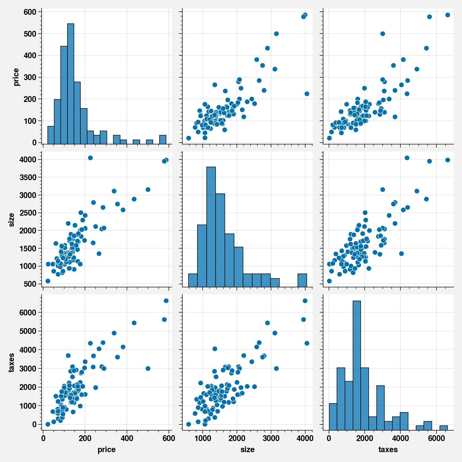
house_df = pd.read_csv("../data/Houses.tsv.gz", sep="\t")
sns.pairplot(house_df[["price", "size", "taxes"]])
<seaborn.axisgrid.PairGrid at 0x7f34688d0ed0>
from statsmodels.stats.anova import anova_lm

fit1 = smf.ols(formula="""price ~ size + new + baths + beds""", data=house_df).fit()
fit2 = smf.ols(
    formula="""price ~ (size + new + baths + beds)**2""", data=house_df
).fit()
fit3 = smf.ols(
    formula="""price ~ (size + new + baths + beds)**3""", data=house_df
).fit()
fit6 = smf.ols(
    formula="""price ~ (size + new + baths + beds)**6""", data=house_df
).fit()

anova_results = anova_lm(fit1, fit2)
anova_results
| df_resid | ssr | df_diff | ss_diff | F | Pr(>F) | |
|---|---|---|---|---|---|---|
| 0 | 95.0 | 279624.077203 | 0.0 | NaN | NaN | NaN |
| 1 | 89.0 | 217916.368647 | 6.0 | 61707.708555 | 4.200377 | 0.000913 |
anova_results = anova_lm(fit2, fit1)
anova_results
| df_resid | ssr | df_diff | ss_diff | F | Pr(>F) | |
|---|---|---|---|---|---|---|
| 0 | 89.0 | 217916.368647 | 0.0 | NaN | NaN | NaN |
| 1 | 95.0 | 279624.077203 | -6.0 | -61707.708555 | 3.494115 | NaN |
anova_results
| df_resid | ssr | df_diff | ss_diff | F | Pr(>F) | |
|---|---|---|---|---|---|---|
| 0 | 89.0 | 217916.368647 | 0.0 | NaN | NaN | NaN |
| 1 | 95.0 | 279624.077203 | -6.0 | -61707.708555 | 3.494115 | NaN |
print(fit6.summary())
                            OLS Regression Results
==============================================================================
Dep. Variable:                  price   R-squared:                       0.804
Model:                            OLS   Adj. R-squared:                  0.771
Method:                 Least Squares   F-statistic:                     24.85
Date:                Tue, 12 Jan 2021   Prob (F-statistic):           3.27e-24
Time:                        23:01:34   Log-Likelihood:                -521.77
No. Observations:                 100   AIC:                             1074.
Df Residuals:                      85   BIC:                             1113.
Df Model:                          14
Covariance Type:            nonrobust
=======================================================================================
                          coef    std err          t      P>|t|      [0.025      0.975]
---------------------------------------------------------------------------------------
Intercept            -195.2928    159.474     -1.225      0.224    -512.369     121.783
size                    0.2512      0.126      2.001      0.049       0.002       0.501
new                   121.6101    119.714      1.016      0.313    -116.412     359.633
baths                 151.0111     73.643      2.051      0.043       4.589     297.433
beds                   39.8477     54.614      0.730      0.468     -68.740     148.435
size:new               -1.8379      1.430     -1.285      0.202      -4.681       1.005
size:baths             -0.1003      0.044     -2.268      0.026      -0.188      -0.012
size:beds              -0.0370      0.035     -1.050      0.297      -0.107       0.033
new:baths             827.9218    717.935      1.153      0.252    -599.525    2255.368
new:beds             -488.2639    407.026     -1.200      0.234   -1297.540     321.012
baths:beds            -39.5669     24.330     -1.626      0.108     -87.942       8.809
size:new:baths          0.3423      0.241      1.423      0.158      -0.136       0.821
size:new:beds           0.7990      0.594      1.345      0.182      -0.382       1.980
size:baths:beds         0.0261      0.011      2.354      0.021       0.004       0.048
new:baths:beds        -75.5298     76.579     -0.986      0.327    -227.788      76.729
size:new:baths:beds    -0.1896      0.135     -1.402      0.164      -0.459       0.079
==============================================================================
Omnibus:                       36.737   Durbin-Watson:                   1.581
Prob(Omnibus):                  0.000   Jarque-Bera (JB):               90.717
Skew:                           1.339   Prob(JB):                     2.00e-20
Kurtosis:                       6.822   Cond. No.                     1.21e+20
==============================================================================

Notes:
[1] Standard Errors assume that the covariance matrix of the errors is correctly specified.
[2] The smallest eigenvalue is 2.09e-30. This might indicate that there are
strong multicollinearity problems or that the design matrix is singular.
4.1. Gamma GLMs for House Selling Price Data
formula = """price ~ size + new + beds + size:new + size:beds"""

response, predictors = dmatrices(formula, house_df, return_type="dataframe")
fit = sm.GLM(
    response, predictors, family=sm.families.Gamma(link=sm.families.links.identity())
).fit()
print(fit.summary())
                 Generalized Linear Model Regression Results
==============================================================================
Dep. Variable:                  price   No. Observations:                  100
Model:                            GLM   Df Residuals:                       94
Model Family:                   Gamma   Df Model:                            5
Link Function:               identity   Scale:                         0.10951
Method:                          IRLS   Log-Likelihood:                -517.66
Date:                Tue, 12 Jan 2021   Deviance:                       10.263
Time:                        23:01:34   Pearson chi2:                     10.3
No. Iterations:                    21
Covariance Type:            nonrobust
==============================================================================
                 coef    std err          z      P>|z|      [0.025      0.975]
------------------------------------------------------------------------------
Intercept     44.3850     48.599      0.913      0.361     -50.867     139.637
size           0.0740      0.040      1.849      0.064      -0.004       0.152
new          -60.0295     65.765     -0.913      0.361    -188.927      68.868
beds         -22.7158     17.632     -1.288      0.198     -57.273      11.841
size:new       0.0538      0.038      1.432      0.152      -0.020       0.127
size:beds      0.0100      0.013      0.796      0.426      -0.015       0.035
==============================================================================
formula = """price ~ size + new + baths + beds"""
response, predictors = dmatrices(formula, house_df, return_type="dataframe")
fit_g1 = sm.GLM(
    response, predictors, family=sm.families.Gamma(link=sm.families.links.identity())
).fit()

formula = """price ~ (size + new + baths + beds)**2"""
response, predictors = dmatrices(formula, house_df, return_type="dataframe")
fit_g2 = sm.GLM(
    response, predictors, family=sm.families.Gamma(link=sm.families.links.identity())
).fit()


def anova_glm(model1, model2):

    # Source: https://static1.squarespace.com/static/58332d815016e1b4077fe29f/t/5d3f1d90ed639e00011487c8/1564417425253/5.2_GLM+-+Comparing+Models-+F+Test+-+Errata.pdf
    df_numerator = model2.df_model - model1.df_model
    f_stat = (model1.deviance - model2.deviance) / (df_numerator * model2.scale)
    df_denominator = model2.fittedvalues.shape[0] - model1.df_model
    p_value = stats.f.sf(f_stat, df_numerator, df_denominator)
    names = ["df_resid", "resid_deviance", "df_diff", "deviance", "F", "Pr(>F)"]
    data = []
    data.append((model1.df_resid, model1.deviance, " ", " ", " ", " "))
    data.append(
        (
            model2.df_resid,
            model2.deviance,
            df_numerator,
            model2.deviance,
            f_stat,
            p_value,
        )
    )
    return pd.DataFrame(data, columns=names)


anova_results = anova_glm(fit_g1, fit_g2)
print(anova_results)
   df_resid  resid_deviance df_diff  deviance         F    Pr(>F)
0        95       10.441719
1        89        9.872775       6  9.872775  0.843782  0.539286
4.2. TODO: Fix the anova_glm output
formula = """price ~ size + new + size:new"""
response, predictors = dmatrices(formula, house_df, return_type="dataframe")
fit = sm.GLM(
    response, predictors, family=sm.families.Gamma(link=sm.families.links.identity())
).fit()
print(fit.summary())
                 Generalized Linear Model Regression Results
==============================================================================
Dep. Variable:                  price   No. Observations:                  100
Model:                            GLM   Df Residuals:                       96
Model Family:                   Gamma   Df Model:                            3
Link Function:               identity   Scale:                         0.11020
Method:                          IRLS   Log-Likelihood:                -519.05
Date:                Tue, 12 Jan 2021   Deviance:                       10.563
Time:                        23:01:34   Pearson chi2:                     10.6
No. Iterations:                    11
Covariance Type:            nonrobust
==============================================================================
                 coef    std err          z      P>|z|      [0.025      0.975]
------------------------------------------------------------------------------
Intercept     -7.4509     12.974     -0.574      0.566     -32.880      17.978
size           0.0945      0.010      9.396      0.000       0.075       0.114
new          -77.9046     64.582     -1.206      0.228    -204.483      48.674
size:new       0.0649      0.037      1.769      0.077      -0.007       0.137
==============================================================================
formula = """price ~ size + new + size:new"""
response, predictors = dmatrices(formula, house_df, return_type="dataframe")
fit = sm.GLM(
    response, predictors, family=sm.families.Gaussian(link=sm.families.links.identity())
).fit()
print(fit.summary())
                 Generalized Linear Model Regression Results
==============================================================================
Dep. Variable:                  price   No. Observations:                  100
Model:                            GLM   Df Residuals:                       96
Model Family:                Gaussian   Df Model:                            3
Link Function:               identity   Scale:                          2703.8
Method:                          IRLS   Log-Likelihood:                -534.97
Date:                Tue, 12 Jan 2021   Deviance:                   2.5957e+05
Time:                        23:01:34   Pearson chi2:                 2.60e+05
No. Iterations:                     3
Covariance Type:            nonrobust
==============================================================================
                 coef    std err          z      P>|z|      [0.025      0.975]
------------------------------------------------------------------------------
Intercept    -22.2278     15.521     -1.432      0.152     -52.649       8.193
size           0.1044      0.009     11.082      0.000       0.086       0.123
new          -78.5275     51.008     -1.540      0.124    -178.501      21.446
size:new       0.0619      0.022      2.855      0.004       0.019       0.104
==============================================================================
formula = """price ~ size + new + size:new"""
response, predictors = dmatrices(formula, house_df, return_type="dataframe")
fit = sm.GLM(
    response, predictors, family=sm.families.Gaussian(link=sm.families.links.identity())
).fit()
print(fit.aic)
1077.9469818936211
formula = """price ~ size + new + beds + baths + size:new + size:beds + new:baths"""
response, predictors = dmatrices(formula, house_df, return_type="dataframe")
fit = sm.GLM(
    response, predictors, family=sm.families.Gaussian(link=sm.families.links.identity())
).fit()
print(fit.aic)
1068.5650280217183