![]()
3. Chapter 3 - Normal Linear Models: Statistical Inference
import warnings

import pandas as pd
import proplot as plot
import seaborn as sns
import statsmodels.api as sm
import statsmodels.formula.api as smf
from patsy import dmatrices
from scipy import stats

warnings.filterwarnings("ignore")
%pylab inline


plt.rcParams["axes.labelweight"] = "bold"
plt.rcParams["font.weight"] = "bold"
Populating the interactive namespace from numpy and matplotlib
stats.f.ppf(0.95, 2, 27) # 0.95 quantile of F dist. with df1=2, df2 =27
3.3541308285291986
1 - stats.f.pdf(3.364131, 2, 27) # right tail probability of non-central F
0.9602934531255635
house_df = pd.read_csv("../data/Houses.tsv.gz", sep="\t")
house_df
| case | taxes | beds | baths | new | price | size | |
|---|---|---|---|---|---|---|---|
| 0 | 1 | 3104 | 4 | 2 | 0 | 279.9 | 2048 |
| 1 | 2 | 1173 | 2 | 1 | 0 | 146.5 | 912 |
| 2 | 3 | 3076 | 4 | 2 | 0 | 237.7 | 1654 |
| 3 | 4 | 1608 | 3 | 2 | 0 | 200.0 | 2068 |
| 4 | 5 | 1454 | 3 | 3 | 0 | 159.9 | 1477 |
| ... | ... | ... | ... | ... | ... | ... | ... |
| 95 | 96 | 990 | 2 | 2 | 0 | 176.0 | 1060 |
| 96 | 97 | 3030 | 3 | 2 | 0 | 196.5 | 1730 |
| 97 | 98 | 1580 | 3 | 2 | 0 | 132.2 | 1370 |
| 98 | 99 | 1770 | 3 | 2 | 0 | 88.4 | 1560 |
| 99 | 100 | 1430 | 3 | 2 | 0 | 127.2 | 1340 |
100 rows × 7 columns
Data Description: Observations on recent homesales in Gainesville, Florida.
pd.concat([house_df.mean(), house_df.std()], axis=1).rename(
    columns={0: "mean", 1: "sd"}
)
| mean | sd | |
|---|---|---|
| case | 50.500 | 29.011492 |
| taxes | 1908.390 | 1235.825663 |
| beds | 3.000 | 0.651339 |
| baths | 1.960 | 0.567112 |
| new | 0.110 | 0.314466 |
| price | 155.331 | 101.262213 |
| size | 1629.280 | 666.941702 |
fit = smf.ols(formula="""price ~ size + new""", data=house_df).fit()
print(fit.summary())
model_residuals = fit.resid
sd_model_residuals = model_residuals.std()
print("Residual SE: {}".format(np.round(sd_model_residuals, 2)))
                            OLS Regression Results
==============================================================================
Dep. Variable:                  price   R-squared:                       0.723
Model:                            OLS   Adj. R-squared:                  0.717
Method:                 Least Squares   F-statistic:                     126.3
Date:                Tue, 12 Jan 2021   Prob (F-statistic):           9.79e-28
Time:                        23:01:27   Log-Likelihood:                -539.05
No. Observations:                 100   AIC:                             1084.
Df Residuals:                      97   BIC:                             1092.
Df Model:                           2
Covariance Type:            nonrobust
==============================================================================
                 coef    std err          t      P>|t|      [0.025      0.975]
------------------------------------------------------------------------------
Intercept    -40.2309     14.696     -2.738      0.007     -69.399     -11.063
size           0.1161      0.009     13.204      0.000       0.099       0.134
new           57.7363     18.653      3.095      0.003      20.715      94.757
==============================================================================
Omnibus:                       12.906   Durbin-Watson:                   1.483
Prob(Omnibus):                  0.002   Jarque-Bera (JB):               29.895
Skew:                           0.370   Prob(JB):                     3.22e-07
Kurtosis:                       5.574   Cond. No.                     6.32e+03
==============================================================================

Notes:
[1] Standard Errors assume that the covariance matrix of the errors is correctly specified.
[2] The condition number is large, 6.32e+03. This might indicate that there are
strong multicollinearity or other numerical problems.
Residual SE: 53.33
Interpretation:
- $H_0: \beta_1 = \beta_2 = 0$ The F-statistic with df1 = 2, df2 = 100-3 = 97 is  126.3 with a low p-value which is not surprising since the null is too strict. In some sense the probability of both the coefficients of size and new being 0 is low.

- Coeff of new: Having "adjusted" for size the coefficient of new is still significant
95%CI for the mean selling price of new homes at the mean size of the new homes, 2354.73 square feet:
prediction = fit.get_prediction({"size": 2354.73, "new": 1})
prediction.summary_frame()
| mean | mean_se | mean_ci_lower | mean_ci_upper | obs_ci_lower | obs_ci_upper | |
|---|---|---|---|---|---|---|
| 0 | 290.963953 | 16.245718 | 258.720701 | 323.207205 | 179.270051 | 402.657856 |
Interpretation: If the model truly holds, the ‘mean_ci_lower’ and ‘mean_ci_upper’ reflects the 95% confidence interval where the population mean will lie. While ‘obs_ci_lower’ and ‘obs_ci_upper’ reflects the 95% CI where the future (predicted) will lie.
3.1. TODO: Derivation of the CI for mean and future y
Also see CrossValidated
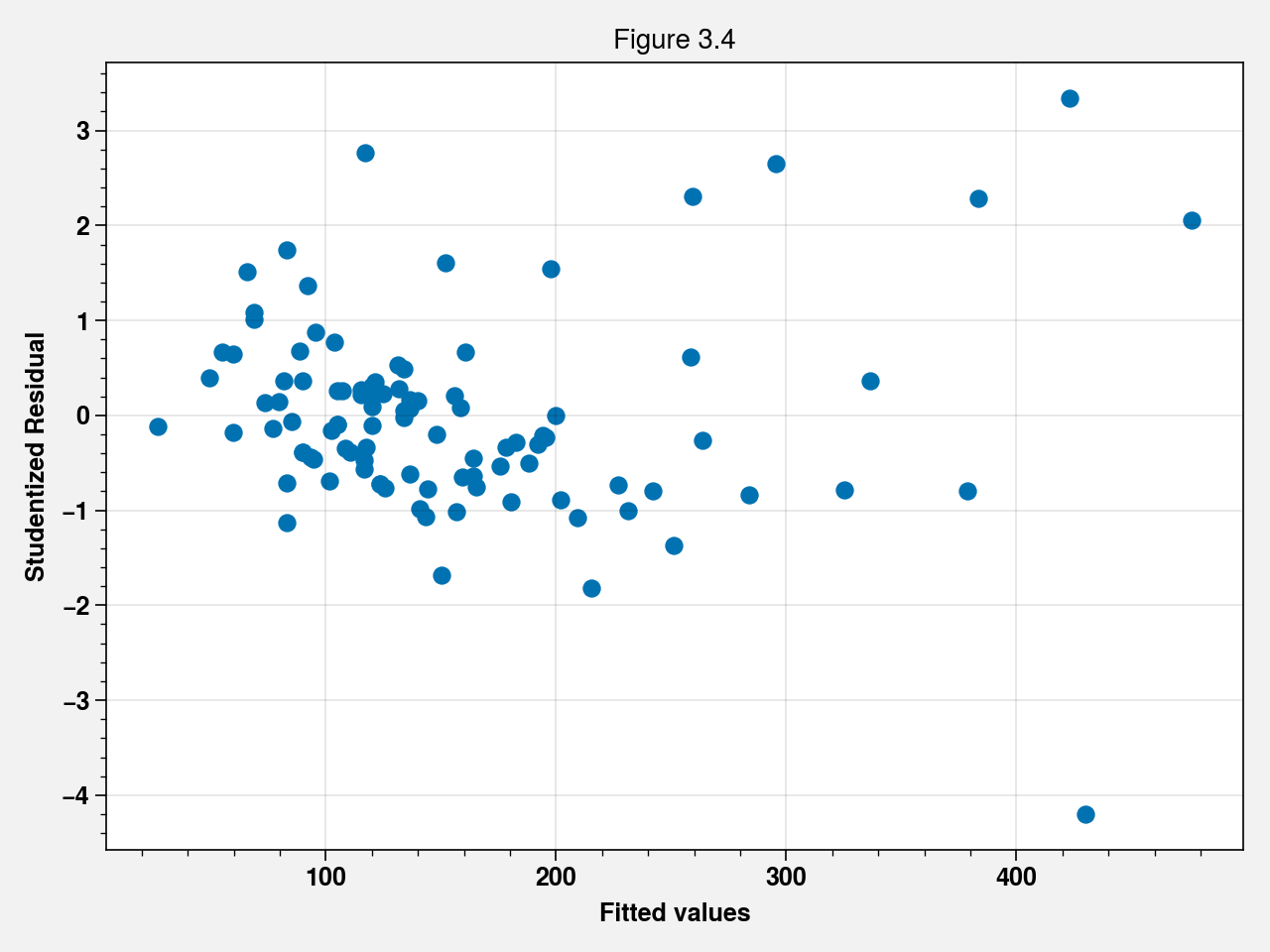
fig, ax = plt.subplots()
ax.scatter(fit.fittedvalues, fit.get_influence().resid_studentized_internal)
ax.set_xlabel("Fitted values")
ax.set_ylabel("Studentized Residual")
ax.set_title("Figure 3.4")
fig.tight_layout()
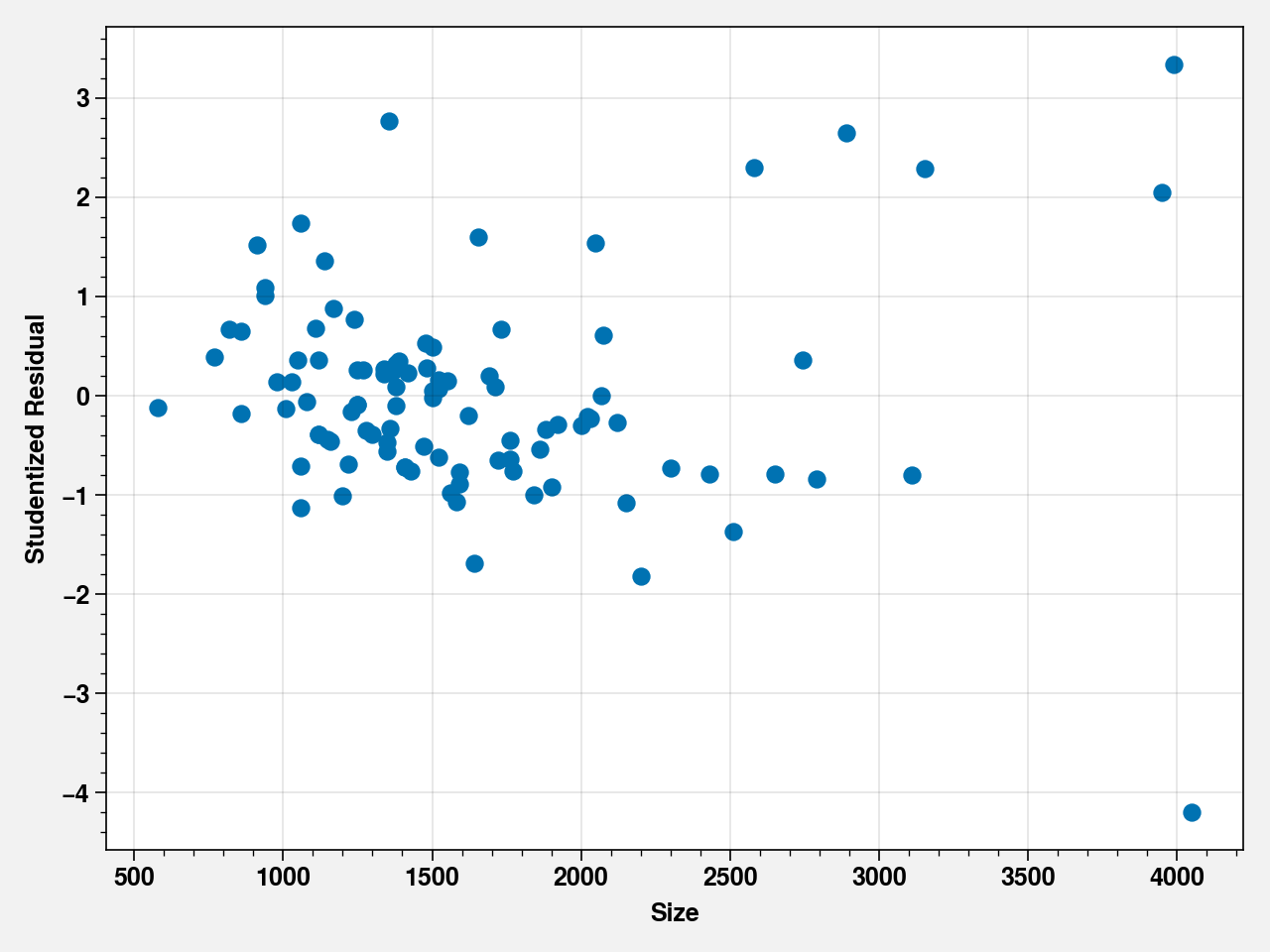
fig, ax = plt.subplots()
ax.scatter(house_df["size"], fit.get_influence().resid_studentized_internal)
ax.set_xlabel("Size")
ax.set_ylabel("Studentized Residual")
fig.tight_layout()
cooks_distance = fit.get_influence().cooks_distance[0]
plt.plot(cooks_distance)
[<matplotlib.lines.Line2D at 0x7fe63ac0eb50>]
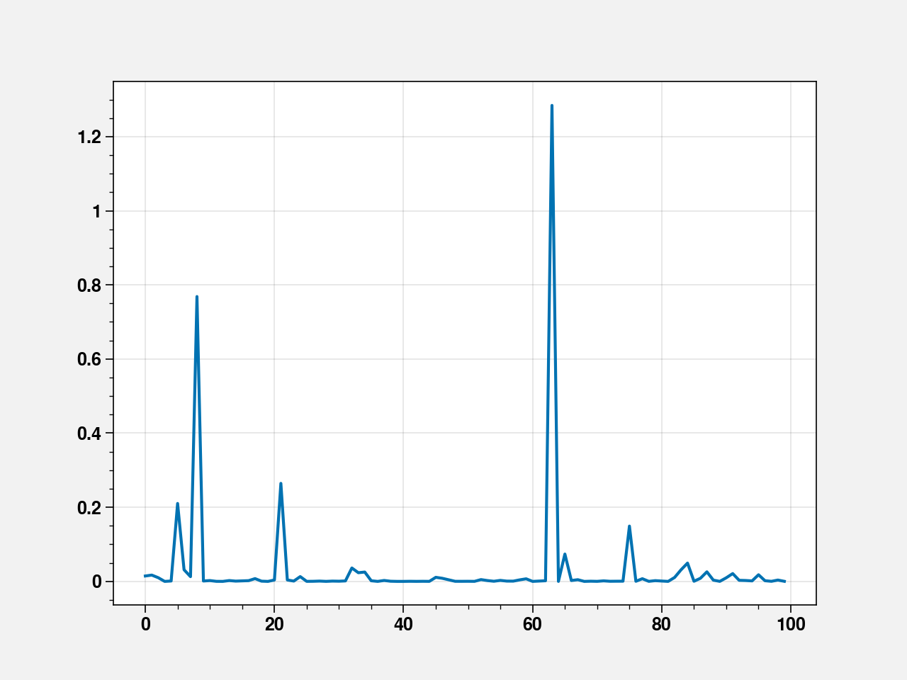
Observation 64 seems influential. Let’s remove it and refit.
fit = smf.ols(
    formula="""price ~ size + new""", data=house_df.loc[cooks_distance < 1]
).fit()
print(fit.summary())
model_residuals = fit.resid
sd_model_residuals = model_residuals.std()
print("Residual SE: {}".format(np.round(sd_model_residuals, 2)))
                            OLS Regression Results
==============================================================================
Dep. Variable:                  price   R-squared:                       0.772
Model:                            OLS   Adj. R-squared:                  0.767
Method:                 Least Squares   F-statistic:                     162.5
Date:                Tue, 12 Jan 2021   Prob (F-statistic):           1.52e-31
Time:                        23:01:28   Log-Likelihood:                -524.21
No. Observations:                  99   AIC:                             1054.
Df Residuals:                      96   BIC:                             1062.
Df Model:                           2
Covariance Type:            nonrobust
==============================================================================
                 coef    std err          t      P>|t|      [0.025      0.975]
------------------------------------------------------------------------------
Intercept    -63.1545     14.252     -4.431      0.000     -91.444     -34.865
size           0.1328      0.009     15.138      0.000       0.115       0.150
new           41.3062     17.327      2.384      0.019       6.913      75.700
==============================================================================
Omnibus:                        8.263   Durbin-Watson:                   1.480
Prob(Omnibus):                  0.016   Jarque-Bera (JB):                7.876
Skew:                           0.640   Prob(JB):                       0.0195
Kurtosis:                       3.520   Cond. No.                     6.42e+03
==============================================================================

Notes:
[1] Standard Errors assume that the covariance matrix of the errors is correctly specified.
[2] The condition number is large, 6.42e+03. This might indicate that there are
strong multicollinearity or other numerical problems.
Residual SE: 48.48
\(R^2\) sees a considerable improvement. Next we check for an interaction:
fit = smf.ols(formula="""price ~ size + new + size:new""", data=house_df.loc[cooks_distance<1]).fit()
print(fit.summary())
model_residuals = fit.resid
sd_model_residuals = model_residuals.std()
print("Residual SE: {}".format(np.round(sd_model_residuals, 2)))
                            OLS Regression Results
==============================================================================
Dep. Variable:                  price   R-squared:                       0.782
Model:                            OLS   Adj. R-squared:                  0.775
Method:                 Least Squares   F-statistic:                     113.7
Date:                Tue, 12 Jan 2021   Prob (F-statistic):           2.52e-31
Time:                        23:01:28   Log-Likelihood:                -521.95
No. Observations:                  99   AIC:                             1052.
Df Residuals:                      95   BIC:                             1062.
Df Model:                           3
Covariance Type:            nonrobust
==============================================================================
                 coef    std err          t      P>|t|      [0.025      0.975]
------------------------------------------------------------------------------
Intercept    -48.2431     15.686     -3.075      0.003     -79.385     -17.102
size           0.1230      0.010     12.536      0.000       0.104       0.142
new          -52.5122     47.630     -1.102      0.273    -147.070      42.046
size:new       0.0434      0.021      2.109      0.038       0.003       0.084
==============================================================================
Omnibus:                       14.139   Durbin-Watson:                   1.508
Prob(Omnibus):                  0.001   Jarque-Bera (JB):               16.134
Skew:                           0.807   Prob(JB):                     0.000314
Kurtosis:                       4.144   Cond. No.                     1.76e+04
==============================================================================

Notes:
[1] Standard Errors assume that the covariance matrix of the errors is correctly specified.
[2] The condition number is large, 1.76e+04. This might indicate that there are
strong multicollinearity or other numerical problems.
Residual SE: 47.39
The increase in \(R^2\) is minimal.
3.2. Simpson’s paradox
Consider adding beds as another explanatory variable.
stats.pearsonr(house_df['beds'], house_df['price'])
(0.39395702205835825, 5.006768706208423e-05)
Thus, beds is modestly correlated with price. Let’s include it in the model and see how the fit changes.
fit = smf.ols(formula="""price ~ size + new""", data=house_df).fit()
print(fit.summary())
model_residuals = fit.resid
sd_model_residuals = model_residuals.std()
print("Residual SE: {}".format(np.round(sd_model_residuals, 2)))
                            OLS Regression Results
==============================================================================
Dep. Variable:                  price   R-squared:                       0.723
Model:                            OLS   Adj. R-squared:                  0.717
Method:                 Least Squares   F-statistic:                     126.3
Date:                Tue, 12 Jan 2021   Prob (F-statistic):           9.79e-28
Time:                        23:01:28   Log-Likelihood:                -539.05
No. Observations:                 100   AIC:                             1084.
Df Residuals:                      97   BIC:                             1092.
Df Model:                           2
Covariance Type:            nonrobust
==============================================================================
                 coef    std err          t      P>|t|      [0.025      0.975]
------------------------------------------------------------------------------
Intercept    -40.2309     14.696     -2.738      0.007     -69.399     -11.063
size           0.1161      0.009     13.204      0.000       0.099       0.134
new           57.7363     18.653      3.095      0.003      20.715      94.757
==============================================================================
Omnibus:                       12.906   Durbin-Watson:                   1.483
Prob(Omnibus):                  0.002   Jarque-Bera (JB):               29.895
Skew:                           0.370   Prob(JB):                     3.22e-07
Kurtosis:                       5.574   Cond. No.                     6.32e+03
==============================================================================

Notes:
[1] Standard Errors assume that the covariance matrix of the errors is correctly specified.
[2] The condition number is large, 6.32e+03. This might indicate that there are
strong multicollinearity or other numerical problems.
Residual SE: 53.33
fit = smf.ols(formula="""price ~ size + new + beds""", data=house_df).fit()
print(fit.summary())
model_residuals = fit.resid
sd_model_residuals = model_residuals.std()
print("Residual SE: {}".format(np.round(sd_model_residuals, 2)))
                            OLS Regression Results
==============================================================================
Dep. Variable:                  price   R-squared:                       0.724
Model:                            OLS   Adj. R-squared:                  0.715
Method:                 Least Squares   F-statistic:                     83.97
Date:                Tue, 12 Jan 2021   Prob (F-statistic):           9.68e-27
Time:                        23:01:28   Log-Likelihood:                -538.78
No. Observations:                 100   AIC:                             1086.
Df Residuals:                      96   BIC:                             1096.
Df Model:                           3
Covariance Type:            nonrobust
==============================================================================
                 coef    std err          t      P>|t|      [0.025      0.975]
------------------------------------------------------------------------------
Intercept    -25.1998     25.602     -0.984      0.327     -76.020      25.620
size           0.1205      0.011     11.229      0.000       0.099       0.142
new           54.8996     19.113      2.872      0.005      16.961      92.838
beds          -7.2927     10.159     -0.718      0.475     -27.458      12.872
==============================================================================
Omnibus:                       13.929   Durbin-Watson:                   1.496
Prob(Omnibus):                  0.001   Jarque-Bera (JB):               41.568
Skew:                           0.277   Prob(JB):                     9.41e-10
Kurtosis:                       6.110   Cond. No.                     8.80e+03
==============================================================================

Notes:
[1] Standard Errors assume that the covariance matrix of the errors is correctly specified.
[2] The condition number is large, 8.8e+03. This might indicate that there are
strong multicollinearity or other numerical problems.
Residual SE: 53.19
Including beds leads to a reduced \(R^2\)!! Thus, once size and new are in the model, it does not help to add beds. Although the marginal effect of beds is positive (as shown by the modest positive correlation), the estimated partial effect of beds is negative. This illustrates Simpson’s paradox.
3.3. Partial Correlation
regress_sizenew_on_price = smf.ols(formula="""price ~ size + new""", data=house_df).fit()
regress_sizenew_on_bed = smf.ols(formula="""beds ~ size + new""", data=house_df).fit()

stats.pearsonr(regress_sizenew_on_price.resid, regress_sizenew_on_bed.resid)
(-0.07307200731424245, 0.4699872574144025)
Partial correlation between selling price and beds. Found using 1) finding the residuals for predicting selling price using size and new 2) finding the residual for predicting beds using size and new and 3) correlating the residuals in 1 and 2.
3.4. TODO: Testing contrats as a general linear hypothesis
from statsmodels.stats.libqsturng import psturng, qsturng

qsturng(0.95, 10, 190)
4.52786052558441
stats.t.ppf(1-0.05/(2*45), 190)
3.3113791139604563